Getting Started

Calyx is an intermediate language and infrastructure for building compilers that generate custom hardware accelerators. These instructions will help you set up the Calyx compiler and associated tools. By the end, you should be able to compile and simulate hardware designs generated by Calyx.

Compiler Installation

There are three possible ways to install Calyx, depending on your goals.

Using Docker

The easiest way is to use the Calyx Docker image that provides a pinned version of the compiler, all frontends, as well as configuration for several tools.

The following commands will fetch the Docker image and start a container with an interactive shell:

docker run -it --rm ghcr.io/calyxir/calyx:latest

The --rm flag will remove the container after you exit the shell. If you want to keep the container around, remove the flag.

You can skip forward to running a hardware design.

Installing the Crate (to use, but not extend, Calyx)

First, install Rust. This should automatically install cargo.

If you want just to play with the compiler, install the calyx crate:

cargo install calyx

This will install the calyx binary which can optimize and compile Calyx programs. You will still need the primitives/core.futil and its accompanying Verilog file library to compile most programs.

Installing from Source (to use and extend Calyx)

First, install Rust. This should automatically install cargo.

Clone the repository:

git clone https://github.com/calyxir/calyx.git

Then build the compiler:

cargo build

You can build and run the compiler with:

cargo build # Builds the compiler
./target/debug/calyx --help # Executes the compiler binary

We recommend installing the git hooks to run linting and formatting checks before each commit:

/bin/sh setup_hooks.sh

You can build the docs by installing mdbook and the callouts preprocessor:

/bin/sh docs/install_tools.sh

Then, run mdbook serve from the project root.

Running Core Tests

The core test suite tests the Calyx compiler's various passes. Install the following tools:

1. runt hosts our testing infrastructure. Install with: cargo install runt
2. jq is a command-line JSON processor. Install with:
   • Ubuntu: sudo apt install jq
   • Mac: brew install jq
   • Other platforms: JQ installation

Build the compiler:

cargo build

Then run the core tests with:

runt -i core

If everything has been installed correctly, this should not produce any failing tests.

Installing the Command-Line Driver

The Calyx driver wraps the various compiler frontends and backends to simplify running Calyx programs. Start at the root of the repository.

Install Flit:

pip3 install flit

Install calyx-py:

cd calyx-py && flit install -s && cd -

Install fud:

flit -f fud/pyproject.toml install -s --deps production

Configure fud:

fud config --create global.root <full path to Calyx repository>

Check the fud configuration:

fud check

fud will report certain tools are not available. This is expected.

Simulation

There are three ways to run Calyx programs: Verilator, Icarus Verilog, and Calyx's native interpreter. You'll want to set up at least one of these options so you can try out your code.

Icarus Verilog is an easy way to get started on most platforms. On a Mac, you can install it via Homebrew by typing brew install icarus-verilog. On Ubuntu, install from source. Then install the relevant fud support by running:

fud register icarus-verilog -p fud/icarus/icarus.py

Type fud check to make sure the new stage is working. Some missing tools are again expected; just pay attention to the report for stages.icarus-verilog.exec.

It is worth saying a little about the alternatives. You could consider:

1. Setting up Verilator for faster performance, which is good for long-running simulations.
2. Using the interpreter to avoid RTL simulation altogether.

Running a Hardware Design

You're all set to run a Calyx hardware design now. Run the following command:

fud e examples/tutorial/language-tutorial-iterate.futil \
  -s verilog.data examples/tutorial/data.json \
  --to dat --through icarus-verilog -v

(Change the last bit to --through verilog to use Verilator instead.)

This command will compile examples/tutorial/language-tutorial-iterate.futil to Verilog using the Calyx compiler, simulate the design using the data in examples/tutorial/data.json, and generate a JSON representation of the final memory state.

Congratulations! You've simulated your first hardware design with Calyx.

Where to go next?

• How can I setup syntax highlighting in my editor?
• How does the language work?
• How do I install Calyx frontends?
• Where can I see further examples with fud?
• How do I write a frontend for Calyx?

Calyx Language Tutorial

This tutorial will familiarize you with the Calyx language by writing a minimal program by hand. Usually, Calyx code will be generated by a frontend. However, by writing the program by hand, you can get familiar with all the basic constructs you need to generate Calyx yourself!

Complete code for each example can be found in the tutorial directory in the Calyx repository.

Get Started

The basic building block of Calyx programs is a component which corresponds to hardware modules (or function definitions for the software-minded).

Here is an empty component definition for main along with an import statement to import the standard library:

import "primitives/core.futil";

component main(@go go: 1) -> (@done done: 1) {
  cells {}
  wires {}
  control {}
}

Put this in a file—you can call it language-tutorial-mem.futil, for example. (The futil file extension comes from an old name for Calyx.)

You can think of a component as a unit of Calyx code roughly analogous to a function: it encapsulates a logical unit of hardware structures along with their control. Every component definition has three sections:

• cells: The hardware subcomponents that make up this component.
• wires: A set of guarded connections between components, possibly organized into groups.
• control: The imperative program that defines the component's execution schedule: i.e., when each group executes.

We'll fill these sections up minimally in the next sections.

A Memory Cell

Let's turn our skeleton into a tiny, nearly no-op Calyx program. We'll start by adding a memory component to the cells:

  cells {
    @external mem = comb_mem_d1(32, 1, 1);
  }

This new line declares a new cell called mem and the primitive component comb_mem_d1 represents a 1D memory. You can see the definition of comb_mem_d1, and all the other standard components, in the primitives/core.futil library we imported.

This one has three parameters: the data width (here, 32 bits), the number of elements (just one), and the width of the address port (one bit).

The @external syntax is an extra bit of magic that allows us to read and write to the memory.

Next, we'll add some assignments to the wires section to update the value in the memory. Insert these lines to put a constant value into the memory:

  wires {
      mem.addr0 = 1'b0;
      mem.write_data = 32'd42;
      mem.write_en = 1'b1;
      done = mem.done;
  }

These assignments refer to four ports on the memory component: addr0 (the address port), write_data (the value we're putting into the memory), write_en (the write enable signal, telling the memory that it's time to do a write), and done (signals that the write was committed). Constants like 32'd42 are Verilog-like literals that include the bit width (32), the base (d for decimal), and the value (42).

Assignments at the top level in the wires section, like these, are "continuous". They always happen, without any need for control statements to orchestrate them. We'll see later how to organize assignments into groups.

The complete program for this section is available under examples/tutorial/language-tutorial-mem.futil.

Compile & Run

We can almost run this program! But first, we need to provide it with data. The Calyx infrastructure can provide data to programs from JSON files. So make a file called something like data.json containing something along these lines:

{
  "mem": {
    "data": [10],
    "format": {
      "numeric_type": "bitnum",
      "is_signed": false,
      "width": 32
    }
  }
}

The mem key means we're providing the initial value for our memory called mem. We have one (unsigned integer) data element, and we indicate the bit width (32 bits).

If you want to see how this Calyx program compiles to Verilog, here's the fud incantation you need:

fud exec language-tutorial-mem.futil --to verilog

Not terribly interesting! However, one nice thing you can do with programs is execute them.

To run our program using Icarus Verilog, do this:

fud exec language-tutorial-mem.futil --to dat --through icarus-verilog \
    -s verilog.data data.json

Using --to dat asks fud to run the program, and the extra -s verilog.data <filename> argument tells it where to find the input data. The --through icarus-verilog option tells fud which Verilog simulator to use (see the chapter about fud for alternatives such as Verilator). Executing this program should print:

{
  "cycles": 1,
  "memories": {
    "mem": [
      42
    ]
  }
}

Meaning that, after the program finished, the final value in our memory was 42.

Note: Verilator may report a different cycle count compared to the one above. As long as the final value in memory is correct, this does not matter.

Add Control

Let's change our program to use an execution schedule. First, we're going to wrap all the assignments in the wires section into a name group:

  wires {
    group the_answer {
      mem.addr0 = 1'b0;
      mem.write_data = 32'd42;
      mem.write_en = 1'b1;
      the_answer[done] = mem.done;
    }
  }

We also need one extra line in the group: that assignment to the_answer[done]. Here, we say that the_answer's work is done once the update to mem has finished. Calyx groups have compilation holes called go and done that the control program will use to orchestrate their execution.

The last thing we need is a control program. Add one line to activate the_answer and then finish:

  control {
    the_answer;
  }

If you execute this program, it should do the same thing as the original group-free version: mem ends up with 42 in it. But now we're controlling things with an execution schedule.

If you're curious to see how the Calyx compiler lowers this program to a Verilog-like structural form of Calyx, you can do this:

fud exec language-tutorial-mem.futil --to calyx-lowered

Notably, you'll see control {} in the output, meaning that the compiler has eliminated all the control statements and replaced them with continuous assignments in wires.

The complete program for this section is available under examples/tutorial/language-tutorial-control.futil.

Add an Adder

The next step is to actually do some computation. In this version of the program, we'll read a value from the memory, increment it, and store the updated value back to the memory.

First, we will add two components to the cells section:

  cells {
    @external(1) mem = comb_mem_d1(32, 1, 1);
    val = std_reg(32);
    add = std_add(32);
  }

We make a register val and an integer adder add, both configured to work on 32-bit values.

Next, we'll create three groups in the wires section for the three steps we want to run: read, increment, and write back to the memory. Let's start with the last step, which looks pretty similar to our the_answer group from above, except that the value comes from the val register instead of a constant:

    group write {
      mem.addr0 = 1'b0;
      mem.write_en = 1'b1;
      mem.write_data = val.out;
      write[done] = mem.done;
    }

Next, let's create a group read that moves the value from the memory to our register val:

    group read {
      mem.addr0 = 1'b0;
      val.in = mem.read_data;
      val.write_en = 1'b1;
      read[done] = val.done;
    }

Here, we use the memory's read_data port to get the initial value out.

Finally, we need a third group to add and update the value in the register:

    group upd {
      add.left = val.out;
      add.right = 32'd4;
      val.in = add.out;
      val.write_en = 1'b1;
      upd[done] = val.done;
    }

The std_add component from the standard library has two input ports, left and right, and a single output port, out, which we hook up to the register's in port. This group adds a constant 4 to the register's value, updating it in place. We can enable the val register with a constant 1 because the std_add component is combinational, meaning its results are ready "instantly" without the need to wait for a done signal.

We need to extend our control program to orchestrate the execution of the three groups. We will need a seq statement to say we want to the three steps sequentially:

  control {
    seq {
      read;
      upd;
      write;
    }
  }

Try running this program again. The memory's initial value was 10, and its final value after execution should be 14.

The complete program for this section is available under examples/tutorial/language-tutorial-compute.futil.

Iterate

Next, we'd like to run our little computation in a loop. The idea is to use Calyx's while control construct, which works like this:

while <value> with <group> {
  <body>
}

A while loop runs the control statements in the body until <value>, which is some port on some component, becomes zero. The with <group> bit means that we activate a given group in order to compute the condition value that determines whether the loop continues executing.

Let's run our memory-updating seq block in a while loop. Change the control program to look like this:

  control {
    seq {
      init;
      while lt.out with cond {
        par {
          seq {
            read;
            upd;
            write;
          }
          incr;
        }
      }
    }
  }

This version uses while, the parallel composition construct par, and a few new groups we will need to define. The idea is that we'll use a counter register to make this loop run a fixed number of times, like a for loop. First, we have an outer seq that invokes an init group that we will write to set the counter to zero. The while loop then uses a new group cond, and it will run while a signal lt.out remains nonzero: this signal will compute counter < 8. The body of the loop runs our old seq block in parallel with a new incr group to increment the counter.

Let's add some cells to our component:

    counter = std_reg(32);
    add2 = std_add(32);
    lt = std_lt(32);

We'll need a new register, an adder to do the incrementing, and a less-than comparator.

We can use these raw materials to build the new groups we need: init, incr, and cond. First, the init group is pretty simple:

    group init {
      counter.in = 32'd0;
      counter.write_en = 1'b1;
      init[done] = counter.done;
    }

This group just writes a zero into the counter and signals that it's done. Next, the incr group adds one to the value in counter using add2:

    group incr {
      add2.left = counter.out;
      add2.right = 32'd1;
      counter.in = add2.out;
      counter.write_en = 1'b1;
      incr[done] = counter.done;
    }

And finally, cond uses our comparator lt to compute the signal we need for our while loop. We use a comb group to denote that the assignments inside the condition can be run combinationally:

    comb group cond {
      lt.left = counter.out;
      lt.right = 32'd8;
    }

By comparing with 8, we should now be running our loop body 8 times.

Try running this program again. The output should be the result of adding 4 to the initial value 8 times, so 10 + 8 × 4.

The complete program for this section is available under examples/tutorial/language-tutorial-iterate.futil.

Take a look at the full language reference for details on the complete language.

Multi-Component Designs

Calyx designs can define and instantiate other Calyx components that themselves encode complex control programs.

As an example, we'll build a Calyx design that uses a simple Calyx component to save a value in a register and use it in a different component.

We define a new component called identity that has an input port in and an output port out.

component identity(in: 32) -> (out: 32) {
  cells {
    r = std_reg(32);
  }
  wires {
    group save {
      r.in = in;
      r.write_en = 1'd1;
      save[done] = r.done;
    }

    // This component always outputs the current value in r
    out = r.out;
  }
  control {
    save;
  }
}

The following line defines a continuous assignment, i.e., an assignment that is always kept active, regardless of the component's control program being active.

    // This component always outputs the current value in r
    out = r.out;

By defining this continuous assignment, we can execute our component and later observe any relevant values.

Next, we can instantiate this component in any other Calyx component. The following Calyx program instantiates the id component and uses it to save a value and observe it.

component main() -> () {
  cells {
    // Instantiate the identity element
    id = identity();
    current_value = std_reg(32);
  }
  wires {
    group run_id {
      // We want to "save" the value 10 inside the identity group.
      id.in = 32'd10;
      // All components have a magic "go" and "done" port added to them.
      // Execute the component.
      id.go = 1'd1;
      run_id[done] = id.done;
    }
    group use_id {
      // We want to "observe" the current value saved in id.
      // The out port on the `id` component always shows the last saved
      // element. We don't need to set the `go` because we're not executing
      // and control.
      current_value.in = id.out;
      current_value.write_en = 1'd1;
      use_id[done] = current_value.done;
    }
  }
  control {
    seq { run_id; use_id; }
  }
}

Our first group executes the component by setting the go signal for the component to high and placing the value 10 on the input port. The second group simply saves the value on the output port. Importantly, we don't have to set the go signal of the component to high because we don't need to save a new value into it. The component executes the two groups in-order.

To see the output from running this component, run the command:

fud e examples/futil/multi-component.futil --to vcd

Passing Cells by Reference

One question that may arise when using Calyx as a backend is how to pass a cell "by reference" between components. In C++, this might look like:

#include <array>
#include <cstdint>

// Adds one to the first element in `v`.
void add_one(std::array<uint32_t, 1>& v) {
  v[0] = v[0] + 1;
}

int main() {
  std::array<uint32_t, 1> x = { 0 };
  add_one(x); // The value at x[0] is now 1.
}

In Calyx, there are two steps to passing a cell by reference:

1. Define the component in a manner such that it can accept a cell by reference.
2. Pass the desired cell by reference.

When we say cell, we mean any cell, including memories of various dimensions and registers.

The language provides two ways of doing this.

The Easy Way: ref Cells

Calyx uses the ref keyword to describe cells that are passed by reference:

component add_one() -> () {
  cells {
    ref mem = comb_mem_d1(32, 4, 3); // A memory passed by reference.
    ...
  }
  ...
}

This component defines mem as a memory that is passed by reference to the component. Inside the component, we can use the cell as usual.

Next, to pass the memory to the component, we use the invoke syntax:

component add_one() -> () { ... }
component main() -> () {
  cells {
    A = comb_mem_d1(32, 4, 3); // A memory that will be passed by reference.
    one = add_one();
    ...
  }
  wires { ... }
  control {
    invoke one[mem = A]()(); // pass A as the `mem` for this invocation.
  }
}

The Calyx compiler will correctly lower the add_one component and the invoke call such that the memory is passed by reference. In fact, any cell can be passed by reference in a Calyx program. Read the next section if you're curious about how this process is implemented.

Multiple memories, multiple components

To understand the power of ref cells, let us work through an example. We will study a relatively simple arbitration logic: the invoker has six memories of size 4 each, but needs to pretend, sometimes simulatenously, that:

1. They are actually two memories of size 12 each.
2. They are actually three memories of size 8 each.

We will do up two components that are designed to receive memories by reference:

component wrap2(i: 32, j: 32) -> () {
  cells {
    // Six memories that will be passed by reference.
    ref mem1 = comb_mem_d1(32, 4, 32);
    // ...
    ref mem6 = comb_mem_d1(32, 4, 32);
    // An answer cell, also passed by reference.
    ref ans = comb_mem_d1(32, 1, 32);
  }
  wires { ... }
  control { ... }
}

and

component wrap3(i: 32, j: 32) -> () {
  cells {
    // Six memories that will be passed by reference.
    ref mem1 = comb_mem_d1(32, 4, 32);
    // ...
    ref mem6 = comb_mem_d1(32, 4, 32);
    // An answer cell, also passed by reference.
    ref ans = comb_mem_d1(32, 1, 32);
  }
  wires { ... }
  control { ... }
}

That is, they have the same signature including input ports, output ports, and ref cells. We have elided the logic, but feel free to explore the source code in Python. You can also generate the Calyx code by running python calyx-py/test/correctness/arbiter_6.py.

Now the invoker has six locally defined memories. By passing these memories to the components above, the invoker is able to wrap the same six memories two different ways, and then maintain two different fictional indexing systems at the same time.

component main() -> () {
  cells {
    // Six memories that will pass by reference.
    @external A = comb_mem_d1(32, 4, 32);
    //...
    @external F = comb_mem_d1(32, 4, 32);

    // Two answer cells that we will also pass.
    @external out2 = comb_mem_d1(32, 1, 32);
    @external out3 = comb_mem_d1(32, 1, 32);

    // Preparing to invoke the components above.
    together2 = wrap2();
    together3 = wrap3();
  }

  wires {
  }

  control {
    seq {
      invoke together2[mem1=A, mem2=B, mem3=C, mem4=D, mem5=E, mem6=F, ans=out2](i=32'd1, j=32'd11)();
      invoke together3[mem1=A, mem2=B, mem3=C, mem4=D, mem5=E, mem6=F, ans=out3](i=32'd2, j=32'd7)();
    }
  }
}

Observe: when "wrapped" into two chunks, \( 0 \le i < 2 \) and \( 0 \le j < 12 \); when wrapped into three chunks, \( 0 \le i < 3 \) and \( 0 \le j < 8 \).

The Hard Way: Without ref Cells

Proceed with caution. We recommend using the ref syntax in almost all cases since it enables the compiler to perform more optimizations.

If we wish not to use ref cells, we can leverage the usual input and output ports to establish a call-by-reference-esque relationship between the calling and called components. In fact, the Calyx compiler takes ref cells as descibed above and lowers them into code of the style described here.

Let us walk through an example.

Worked example: mem_cpy

In the C++ code above, we've constructed an "l-value reference" to the array, which essentially means we can both read and write from x in the function add_one.

Now, let's allow similar functionality at the Calyx IR level. We define a new component named add_one which represents the function above. However, we also need to include the correct ports to both read and write to x:

Since we're both reading and writing from x, we'll include the union of the columns above:

component add_one(x_done: 1, x_read_data: 32) ->
                 (x_write_data: 32, x_write_en: 1, x_addr0: 1) {

One tricky thing to note is where the ports belong, i.e. should it be an input port or an output port of the component? The way to reason about this is to ask whether we want to receive signal from or send signal to the given wire. For example, with read_data, we will always be receiving signal from it, so it should be an input port. Conversely, address ports are used to mark where in memory we want to access, so those are used as output ports.

We then simply use the given ports to both read and write to the memory passed by reference. Note that we've split up the read and write to memory x in separate groups, to ensure we can schedule them sequentially in the execution flow. We're also using the exposed ports of the memory through the component interface rather than, say, x.write_data.

    group read_from_x {
      x_addr0 = 1'd0;            // Set address port to zero.
      tmp_reg.in = x_read_data;  // Read the value at address zero.
      tmp_reg.write_en = 1'd1;
      read_from_x[done] = tmp_reg.done;
    }
    group write_to_x {
      x_addr0 = 1'd0;            // Set address port to zero.
      add.left = one.out;
      add.right = tmp_reg.out;   // Saved value from previous read.

      x_write_data = add.out;    // Write value to address zero.
      x_write_en = 1'd1;         // Set write enable signal to high.

      write_to_x[done] = x_done; // The group is done when the write is complete.
    }

Bringing everything back together, the add_one component is written accordingly:

component add_one(x_done: 1, x_read_data: 32) ->
                 (x_write_data: 32, x_write_en: 1, x_addr0: 1) {
  cells {
    one = std_const(32, 1);
    add = std_add(32);
    tmp_reg = std_reg(32);
  }
  wires {
    group read_from_x {
      x_addr0 = 1'd0;            // Set address port to zero.
      tmp_reg.in = x_read_data;  // Read the value at address zero.
      tmp_reg.write_en = 1'd1;
      read_from_x[done] = tmp_reg.done;
    }
    group write_to_x {
      x_addr0 = 1'd0;            // Set address port to zero.
      add.left = one.out;
      add.right = tmp_reg.out;   // Saved value from previous read.

      x_write_data = add.out;    // Write value to address zero.
      x_write_en = 1'd1;         // Set write enable signal to high.

      write_to_x[done] = x_done; // The group is done when the write is complete.
    }
  }
  control {
    seq { read_from_x; write_to_x; }
  }
}

The final step is creating a main component from which the original component will be invoked. In this step, it is important to hook up the proper wires in the call to invoke to the corresponding memory you'd like to read and/or write to:

  control {
    invoke add_one0(x_done = x.done, x_read_data = x.read_data)
                   (x_write_data = x.write_data, x_write_en = x.write_en, x_addr0 = x.addr0);
  }

This gives us the main component:

component main() -> () {
  cells {
    add_one0 = add_one();
    @external(1) x = comb_mem_d1(32, 1, 1);
  }
  wires {
  }
  control {
    invoke add_one0(x_done = x.done, x_read_data = x.read_data)
                   (x_write_data = x.write_data, x_write_en = x.write_en, x_addr0 = x.addr0);
  }
}

To see this example simulated, run the command:

fud e examples/futil/memory-by-reference/memory-by-reference.futil --to dat \
-s verilog.data examples/futil/memory-by-reference/memory-by-reference.futil.data

Multi-dimensional Memories

Not much changes for multi-dimensional arrays. The only additional step is adding the corresponding address ports. For example, a 2-dimensional memory will require address ports addr0 and addr1. More generally, an N-dimensional memory will require address ports addr0, ..., addr(N-1).

Multiple Memories

Similarly, multiple memories will just require the ports to be passed for each of the given memories. Here is an example of a memory copy (referred to as mem_cpy in the C language), with 1-dimensional memories of size 5:

import "primitives/core.futil";
import "primitives/memories/comb.futil";
component copy(dest_done: 1, src_read_data: 32, length: 3) ->
              (dest_write_data: 32, dest_write_en: 1, dest_addr0: 3, src_addr0: 3) {
  cells {
    lt = std_lt(3);
    N = std_reg(3);
    add = std_add(3);
  }
  wires {
    comb group cond {
      lt.left = N.out;
      lt.right = length;
    }
    group upd_index<"static"=1> {
      add.left = N.out;
      add.right = 3'd1;
      N.in = add.out;
      N.write_en = 1'd1;
      upd_index[done] = N.done;
    }
    group copy_index_N<"static"=1> {
      src_addr0 = N.out;
      dest_addr0 = N.out;
      dest_write_en = 1'd1;
      dest_write_data = src_read_data;
      copy_index_N[done] = dest_done;
    }
  }
  control {
    while lt.out with cond {
      seq {
        copy_index_N;
        upd_index;
      }
    }
  }
}

component main() -> () {
  cells {
    @external(1) d = comb_mem_d1(32,5,3);
    @external(1) s = comb_mem_d1(32,5,3);
    length = std_const(3, 5);
    copy0 = copy();
  }
  wires {
  }
  control {
    seq {
      invoke copy0(dest_done=d.done, src_read_data=s.read_data, length=length.out)
                  (dest_write_data=d.write_data, dest_write_en=d.write_en, dest_addr0=d.addr0, src_addr0=s.addr0);
    }
  }
}

Calyx Language Reference

Top-Level Constructs

Calyx programs are a sequence of import statements followed by a sequence of extern statements or component definitions.

import statements

import "<path>" has almost exactly the same semantics to that of #include in the C preprocessor: it copies the code from the file at path into the current file.

extern definitions

extern definitions allow Calyx programs to link against arbitrary RTL code. An extern definition looks like this:

extern "<path>" {
  <primitives>...
}

<path> should be a valid file system path that points to a Verilog module that defines the same names as the primitives defined in the extern block. When run with the -b verilog flag, the Calyx compiler will copy the contents of every such Verilog file into the generated output.

primitive definitions

The primitive construct allows specification of the signature of an external Verilog module that the Calyx program uses. It has the following syntax:

[comb] primitive name<attributes>[PARAMETERS](ports) -> (ports);

The syntax for primitives resembles that for components, with some additional pieces:

• The comb keyword signals that the primitive definition wraps purely combinational RTL code. This is useful for certain optimizations.
• Attributes specify useful metadata for optimization.
• PARAMETERS are named compile-time (metaprogramming) parameters to pass to the Verilog module definition. The primitive definition lists the names of integer-valued parameters; the corresponding Verilog module definition should have identical parameter declarations. Calyx code provides values for these parameters when instantiating a primitive as a cell.
• The ports section contain sized port definitions that can either be positive number or one of the parameter names.

For example, the following is the signature of the std_reg primitive from the Calyx standard library:

primitive std_reg<"state_share"=1>[WIDTH](
  @write_together(1) @data in: WIDTH,
  @write_together(1) @interval(1) @go write_en: 1,
  @clk clk: 1,
  @reset reset: 1
) -> (
  @stable out: WIDTH,
  @done done: 1
)

The primitive defines one parameter called WIDTH, which describes the sizes for the in and the out ports.

Inlined Primitives

Inlined primitives do not have a corresponding Verilog file, and are defined within Calyx. The Calyx backend then converts these definitions into Verilog.

For example, the std_unsyn_mult primitive is inlined:

comb primitive std_unsyn_mult<"share"=1>[WIDTH](left: WIDTH, right: WIDTH) -> (out: WIDTH) {
  assign out = left * right;
};

This can be useful when a frontend needs to generate both Calyx and Verilog code at the same time. The backend ensures that the generated Verilog module has the correct signature.

Calyx Components

Components are the primary encapsulation unit of a Calyx program. They look like this:

component name<attributes>(ports) -> (ports) {
  cells { ... }
  wires { ... }
  control { ... }
}

Like primitive definitions, component signatures consist of a name, an optional list of attributes, and input/output ports. Unlike primitives, component definitions do not have parameters; ports must have a concrete (integer) width. A component encapsulates the control and the hardware structure that implements a hardware module.

Well-formedness: The control program of a component must take at least one cycle to finish executing.

Combinational Components

Using the comb keyword before a component definition marks it as a purely combinational component:

comb component add(left: 32, right: 32) -> (out: 32) {
  cells {
    a = std_add(32);
  }
  wires {
    a.left = left;
    a.right = right;
    out = a.out;
  }
}

A combinational component does not have a control section, can only use other comb components or primitives, and performs its computation combinationally.

Ports

A port definition looks like this:

[@<attr>...] <name>: <width>

Ports have a bit width but are otherwise untyped. They can also include optional attributes. For example, this component definition:

component counter(left: 32, right: 32) -> (@stable out0: 32, out1: 32) { .. }

defines two input ports, left and right, and two output ports, out0 and out1. All four ports are 32-bit signals. Additionally, the out0 port has the attribute @stable.

cells

A component's cells section instantiates a set of sub-components. It contains a list of declarations with this syntax:

[ref]? <name> = <comp>(<param...>);

Here, <comp> is the name of an existing primitive or component definition, and <name> is the fresh, local name of the instance. The optional ref parameter turns the cell into a by-reference cell. Parameters are only allowed when instantiating primitives, not Calyx-defined components.

For example, the following definition of the counter component instantiates a std_add and std_reg primitive as well as a foo Calyx component

component foo() -> () { ... }
component counter() -> () {
  cells {
    r = std_reg(32);
    a = std_add(32);
    f = foo();
  }
  wires { ... }
  control { ... }
}

When instantiating a primitive definition, the parameters are passed within the parenthesis. For example, we pass 32 for the WIDTH parameter of the std_reg in the above instantiation. Since an instantiation of a Calyx component does not take any parameters, the parameters are always empty.

The wires Section

A component's wires section contains guarded assignments that connect ports together. The assignments can either appear at the top level, making them continuous assignments, or be organized into named group and comb group definitions.

Guarded Assignments

Assignments connect ports between two cells together, with this syntax:

<cell>.<port> = [<guard> ?] <cell>.<port>;

The left-hand and right-hand side are both port references, which name a specific input or output port within a cell declared within the same component. The optional guard condition is a logical expression that determines whether the connection is active.

For example, this assignment:

r.in = add.out;

unconditionally transfers the value from a port named out in the add cell to r's in port.

Assignments are simultaneous and non-blocking. When a block of assignments runs, they all first read their right-hand sides and then write into their left-hand sides; they are not processed in order. The result is that the order of assignments does not matter. For example, this block of assignments:

r.in = add.out;
add.left = y.out;
add.right = z.out;

is a valid way to take the values from registers y and z and put the sum into r. Any permutation of these assignments is equivalent.

Guards

An assignment's optional guard expression is a logical expression that produces a 1-bit value, as in these examples:

r.in = cond.out ? add.out;
r.in = !cond.out ? 32'd0;

Using guards, Calyx programs can assign multiple different values to the same port. Omitting a guard expression is equivalent to using 1'd1 (a constant "true") as the guard.

Guards can use the following constructs:

• port: A port access on a defined cell, such as cond.out, or a literal, such as 3'd2.
• port op port: A comparison between values on two ports. Valid instances of op are: >, <, >=, <=, ==
• !guard: Logical negation of a guard value
• guard | guard: Disjunction between two guards
• guard & guard: Conjunction of two guards

Well-formedness: For each input port on the LHS, only one guard should be active in any given cycle during the execution of a Calyx program.

Continuous Assignments

When an assignment appears directly inside a component's wires section, it is called a continuous assignment and is permanently active, even when the control program of the component is inactive.

group definitions

A group is a way to name a set of assignments that together represent some meaningful action:

group name<attributes> {
  assignments...
  name[done] = done_cond;
}

Assignments within a group can be reasoned about in isolation from assignments in other groups. Unlike continuous assignments, a group's encapsulated assignments only execute as dictated by the control program. This means that seemingly conflicting writes to the same ports are allowed:

group foo {
  r.in = 32'd10;
  foo[done] = ...;
}
group bar {
  r.in = 32'd22;
  bar[done] = ...;
}

However, group assignments must not conflict with continuous assignments defined in the component:

group foo {
  r.in = 32'd10; ... // Malformed because it conflicts with the write below.
  foo[done] = ...
}
r.in = 32'd50;

Groups can take any (nonzero) number of cycles to complete. To indicate to the outside world when their execution has completed, every group has a special done signal, which is a special port written as <group>[done]. The group should assign 1 to this port to indicate that its execution is complete.

Groups can have an optional list of attributes.

Well-formedness: All groups are required to run for at least one cycle. (Sub-cycle logic should use comb group instead.)

comb group definitions

Combinational groups are a restricted version of groups which perform their computation purely combinationally and therefore run for "less than one cycle":

comb group name<attributes> {
  assignments...
}

Because their computation is required to run for less than a cycle, comb group definitions do not specify a done condition.

Combinational groups cannot be used within normal control operators. Instead, they only occur after the with keyword in a control program.

The Control Operators

The control section of a component contains an imperative program that describes the component's behavior. The statements in the control program consist of the following operators:

Group Enable

Simply naming a group in a control statement, called a group enable, executes the group to completion. This is a leaf node in the control program.

invoke

invoke acts like the function call operator for Calyx and has the following syntax:

invoke instance[ref cells](inputs)(outputs) [with comb_group];

• instance is the name of the cell instance that needs to be invoked.
• inputs and outputs define connections for a subset of input and output ports of the instance.
• The with comb_group section is optional and names a combinational group that is active during the execution of the invoke statement.
• ref cells is a list of cell names to pass to the invoked component's required cell reference. (It can be omitted if the invoked component contains no cell references.)

Invoking an instance runs its control program to completion before returning. Any Calyx component or primitive that implements the go-done interface can be invoked. Like the group enable statement, invoke is a leaf node in the control program.

seq

The syntax for sequential composition is:

seq { c1; ...; cn; }

where each ci is a nested control statement. Sequences run the control programs c1...cn in sequence, guaranteeing that each program runs fully before the next one starts executing. seq does not provide any cycle-level guarantees on when a succeeding group starts executing after the previous one finishes.

par

The syntax for parallel composition is:

par { c1; ...; cn; }

The statement runs the nested control programs c1...cn in parallel, guaranteeing that each program only runs once. par does not provide any guarantees on how the execution of child programs is scheduled. It is therefore not safe to assume that all children begin execution at the same time.

Well-formedness: The assignments in the children c1...cn should never conflict with each other.

if

The syntax is:

if <port> [with comb_group] {
  true_c
} else {
  false_c
}

The conditional execution runs either true_c or false_c using the value of <port>. The optional with comb_group syntax allows running a combinational group that computes the value of the port.

Well-formedness: The combinational group is considered to be running during the entire execution of the control program and therefore should not have conflicting assignments with either true_c or false_c.

while

The syntax is:

while <port> [with comb_group] {
  body_c
}

Repeatedly executes body_c while the value on port is non-zero. The optional with comb_group enables a combinational group that computes the value of port.

Well-formedness: The combinational group is considered active during the execution of the while loop and therefore should not have conflicting assignments with body_c.

repeat

The syntax is:

repeat <num_repeats> {
  body_c
}

Repeatedly executes the control program body_c num_repeat times in a row.

The go-done Interface

By default, Calyx components implement a one-sided ready-valid interface called the go-done interface. During compilation, the Calyx compiler will add an input port marked with the attribute @go and an output port marked with the attribute @done to the interface of the component:

component counter(left: 32, right: 32, @go go: 1) -> (out: 32, @done done: 1)

The interface provides a way to trigger the control program of the counter using assignments. When the go signal of the component is set to 1, the control program starts executing. When the component sets the done signal to 1, its control program has finished executing.

Well-formedness: The go signal to the component must remain set to 1 while the done signal is not 1. Lowering the go signal before the done signal is set to 1 will lead to undefined behavior.

The clk and reset Ports

The compiler also adds special input ports marked with @clk and @reset to the interface. By default, Calyx components are not allowed to look at or use these signals. They are automatically threaded to any primitive that defines @clk or @reset ports.

Advanced Concepts

ref cells

Calyx components can specify that a cell needs to be passed "by reference":

// Component that performs mem[0] += 1;
component update_memory() -> () {
  cells {
    ref mem = comb_mem_d1(...)
  }
  wires { ... }
  control { ... }
}

When invoking such a component, the calling component must provide a binding for each defined cell:

component main() -> () {
  cells {
    upd = update_memory();
    m1 = comb_mem_d1(...);
    m2 = comb_mem_d2(...);
  }
  wires { ... }
  control {
    seq {
      invoke upd[mem=m1]()(); // Pass `m1` by reference
      invoke upd[mem=m2]()(); // Pass `m2` by reference
    }
  }
}

As the example shows, each invocation can take different bindings for each ref cell. In the first invocation, we pass in the concrete cell m1 while in the second we pass in m2. See the tutorial for longer example on how to use this feature.

Subtyping for ref cells

When providing bindings for ref cells, one must provide a concrete cell that is a subtype of the ref cell. A cell a is a subtype of cell b if the component defining a has at least the same ports as the component defining b.

Consider the following component definitions:

component b(in_1 : 1) -> (out_1 : 1) {
    // cells, wires, and control blocks
}

component a(in_1 : 1, in_2 : 1) -> (out_1 : 1, out_2 : 1){
    // cells, wires, and control blocks
}

Because the component definition of a has the ports in_1 and out_1, a concrete cell of a can be bound to a ref cell of component b:

//Expects a `ref` cell of component `b`
component c() -> () {
    cells{
        ref b1 = b();
    }
    wires{...}
    control{...}
}


component main() -> () {
  cells {
      c_cell = c();
      b_cell = b();
      a_cell = a(); //recall `a` is a subtype of `b`
  }
  wires { ... }
  control {
    seq {
      // Pass `b_cell` by reference. Both are `b1` and `b_cell` are defined by the component `b`
      invoke c[b1=b_cell]()(); 
      // Pass `a_cell` by reference. The `ref` cell and concrete cell are defined by different components,
      // but this is allowed because `a` is a subtype of `b`.
      invoke c[b1=a_cell]()();
    }
  }
}

Ports are considered to be equal with respect to subtyping if they have the same name, width, direction, and attributes.

Note: The notion of subtyping described above, that only checks for port equivalence between components, is incomplete. A complete, correct definition of subtyping would require that for a to be a subtype of b, for every ref cell expected in a, component b must expect a ref cell that is a subtype of the associated ref cell in a (note that the relationship between these nested ref cells is opposite the relationship of a and b).

Because nested ref cells are not currently allowed in Calyx, this is not a problem in practice.

Data Format

Calyx's fud-based workflows specifies a JSON-based data format which can be used with software simulators.

External memories

First, a Calyx program must mark memories using the @external attribute to tell the compiler that the memory is used as either an input or an ouput.

component main() {
    cells {
        @external ext = comb_mem_d1(...);
        internal = comb_mem_d1(...);
    }
}

In the above program, the memory ext will be assumed to be an input-output memory by the compiler while internal is considered to be an internal memory. For all external memories, the compiler will generate code to read initial values and dump out final values. The external attribute is recognized for all the std_mem and seq_mem primitives. The @external attribute can only be used on the top-level component.

When the --synthesis flag is passed to the compiler, this behavior is disabled and instead the memories are turned into ports on the top-level component.

The Data Format

The JSON-based data format allows us to provide inputs for a memory and specify how the values should be interpreted:

{
  "mem": {
    "data": [10],
    "format": {
      "numeric_type": "bitnum",
      "is_signed": false,
      "width": 32
    }
  }
}

The data field represents the initial data for the memory and can use mutlidimensional arrays to describe it. For example, the following is the initial data for a two-dimensional (comb_mem_d2) memory:

{
    "data": [ [1, 2], [3, 4] ],
    "format": {...}
}

The format specifier tells fud how to interpret the values in the data field. The original program specifies that all values should be treated as 32-bit, unsigned values.

In order to specify fixed-point values, we must specify both the total width and fraction widths:

"root": {
  "data": [
      0.0
  ],
  "format": {
      "numeric_type": "fixed_point",
      "is_signed": false,
      "width": 32,
      "frac_width": 16
  }
}

The format states that all values have a fractional width of 16-bits while the remainder is used for the integral part.

Note: fud requires that for each memory marked with the @external attribute in the program.

Using fud

All software simulators supported by fud, including Verilator and Icarus Verilog, as well as the Calyx interpreter can use this data format. To pass a JSON file with initial values, use the -s verilog.data flag:

# Use Icarus Verilog
fud e --to dat --through icarus-verilog <CALYX FILE> -s verilog.data <JSON>
# Use Verilator
fud e --to dat --through verilog <CALYX FILE> -s verilog.data <JSON>
# Use the Calyx Interpreter
fud e --to interpreter-out <CALYX FILE> -s verilog.data <JSON>

Generating Random Values

Often times, it can be useful to automatically generate random values for a large memory. The data-gen tool takes a Calyx program as an input and automatically generates random values for each memory marked with @external in the above data format.

Static Timing

The features discussed below have been available since Calyx version 0.2.1.

By default, Calyx programs use a latency-insensitive, or dynamic, model of computation. This means that the compiler does not know, track, or guarantee the number of cycles it takes to perform a computation or run a control operator. This is in contrast to a latency-sensitive, or static, model of computation, where the number of cycles a component needs is known to, and honored by, the compiler.

In general, latency-insensitivity makes it easier to compose programs. It grants the compiler freedom to schedule operators however it wants, as long as the schedule meets the program's dataflow constraints. It also prevents code from implicitly depending on the state of other code running in parallel.

However, there are two drawbacks to this approach. First, the generated hardware may not be efficient: if the compiler does not know how long computations take, it must schedule them conservatively. Second, it is impossible for latency-insensitive programs to interact with latency-sensitive hardware implemented in RTL; this means that the use of black-box hardware designs requires costly handshaking logic at the interface.

To address these issues, Calyx provides a static qualifier that modifies components and groups, along with static variants of other control operators.

Broadly, the static qualifier is a promise to the compiler that the specifed component or group will take exactly the specified number of cycles to execute. The compiler is free to take advantage of this promise to generate more efficient hardware. In return, the compiler must access out-ports of static components only after the specified number of cycles have passed, or risk receiving incorrect results.

Static Constructs in the Calyx IL

We will now discuss the static constructs available in the Calyx IL, along with the guarantees they come with.

Static Components

Briefly consider a divider component, std_div_pipe, which divides the value left by the value right and puts the result, which is in two parts, in two out ports. This component is dynamic; its latency is unknown.

primitive std_div_pipe[W](go: 1, left: W, right: W) -> (out_remainder: W, out_quotient: W, done: 1);

A client of the divider must pass two inputs left and right, raise the go signal, and wait for the component itself to raise its done signal. The client can then read the result from the two out ports. That is, it obeys the go-done interface.

Compare this to a multiplier component, std_mult_pipe, which has a similar signature but whose latency is known to be three cycles. We declare it as follows:

static<3> primitive std_mult_pipe[W](go: 1, left: W, right: W) -> (out: W);

The fact that the multiplier has one out port while the divider has two is not relevant to the discussion.

The differences that do matter are:

• The static qualifier is used to declare the component as static and to specify its latency (3 cycles).
• The done port is absent from the multiplier's signature.

A client of the multiplier must pass two inputs and raise the go signal as before. However, the client need not then wait for the component to indicate completion. The client can simply and safely assume that the result will be available after 3 cycles. This is a guarantee that the author of the component has made to the client, and the client is free to take advantage of it.

Static Groups and Relative Timing Guards

Much like components, groups can be declared as static. Since groups are just unordered sets of assignments, it pays to have a little more control over the scheduling of the assignments within a group. To this end, static groups have a unique feature that ordinary dynamic groups do not: relative timing guards.

Consider this group, which multiplies 6 and 7 and stores the result in ans.

static<4> group mult_and_store {
  mult.left = %[0:3] ? 6;
  mult.right = %[0:3] ? 7;
  mult.go = %[0:3] ? 1;
  ans.in = %3 ? mult.out;
  ans.write_en = %3 ? 1;
}

The static<4> qualifier specifies that the group should take 4 cycles to execute.

The first three assignments are guarded (using the standard ? separator) by the relative timing guard %[0:3]. In general, a relative timing guard %[i:j] is true in the half-open interval from cycle i to cycle j of the group’s execution and false otherwise.

In our case, the first three assignments execute only in the first three cycles of the group's execution. The guard %3, which we see immediately afterwards, is syntactic sugar for %[3:4]. We have used it in this case to ensure that the last two assignments execute only in the last cycle of the group's execution.

Static Control Operators

Calyx provides static variants of each of its control operators. While dynamic commands may contain both static and dynamic children, static commands must only have static children. In the examples below, assume that A5, B6, C7, and D8 are static groups with latencies 5, 6, 7, and 8, respectively.

static seq, a static version of seq

If we have static seq { A5; B6; C7; D8; }, we can guarantee that the latency of the entire operation is the sum of the latencies of its children: 5 + 6 + 7 + 8 = 26 cycles in this case. We can also guarantee that each child will begin executing exactly one cycle after the previous child has finished. In our case, for example, B6 will begin executing exactly one cycle after A5 has finished.

static par, a static version of par

If we have static par { A5; B6; C7; D8; }, we can guarantee that the latency of the entire operation is the maximum of the latencies of its children: 8 cycles in this case. Further, all the children of a static par are guaranteed to begin executing at the same time. The children can rely on this "lockstep" behavior and can communicate with each other. Inter-thread communication of this sort is undefined behavior in a standard, dynamic, par.

As a corollary, consider this useful trick in the case when we need A5 and D8 to run in parallel, but we do not want them to start at the same time. Instead, in order to support some inter-thread communication, we want A5 to start three cycles after D8.

static<3> group dummy_group { }

static par {
  static seq { dummy_group; A5; }
  D8;
}

We have not elided the body of dummy_group; it can literally be left blank. During compilation, no hardware will be generated for dummy_group. It is simply a placeholder to delay the start of A5 by three cycles.

static if, a static version of if

If we have static if { A5; B6; }, we can guarantee that the latency of the entire operation is the maximum of the latencies of its children: 6 cycles in this case.

static repeat, a static version of repeat

If we have static repeat 7 { B6; }, we can guarantee that the latency of the entire operation is the product of the number of iterations and the latency of its child: 7 × 6 = 42 cycles in this case. The body of a static repeat is guaranteed to begin executing exactly one cycle after the previous iteration has finished.

Calyx's while loop is unbouded and so it does not have a static variant.

static invoke, a static version of invoke

Its latency is the latency of the invoked cell.

Experimental: Synchronization

Calyx's default semantics do not admit any predictable form of language-level synchronization in presence of parallelism. We're currently experimenting with a suite of new primitives that add synchronization to the language.

@sync attribute

Motivation

Consider the following control program in calyx:

    par {
      /// thread A
      while lt.out with comp {
        seq {
          incr_idx;
          add_r_to_accm;
        }
      }

      /// thread B
      while lt.out with comp {
        seq {
          incr_r;
        }
      }
    }

where groups add_r_to_accm and incr_r reads value and increments value in register r, respectively, as indicated by their names.

Because calyx does not make any guarantee of the order of execution for threads running in parallel, it is impossible for us to determine which thread will access r first for each iteration.

Nondeterminism when running parallel threads is beneficial on the compiler's end, as it will give the compiler more freedom for optimization. However, we sometimes do want to give parallel threads a measure of ordering while still taking advantage of the performance boost of parallelism. The @sync attribute allows us to do that.

Using the @sync attribute

Now we want to modify the program above so that in every iteration, thread A always reads after thread B finishes incrementing using the @sync attribute with the following:

    par {
      // thread A
      while lt.out with comp {
        seq {
          incr_idx;
          @sync(1);
          add_r_to_accm;
          @sync(2);
        }
      }

      // thread B
      while lt.out with comp {
        seq {
          incr_r;
          @sync(1);
          @sync(2);
        }
      }
    }

First and foremost, always remember to import "primitives/sync.futil" when using the @sync attribute.

The @sync syntax can only be marked with empty statements. @sync means that the thread marked with a certain value, now called barrier index, for this attribute, must stop and wait for all other threads marked with the same barrier index to arrive, at which point they can proceed.

In the modified program above, we see that incr_idx and incr_r must both finish in order for either thread to go forth. Because add_r_to_accm is executed after incr_idx in thread A, we know that in each iteration, incr_r will always increment r before add_r_to_accm reads it. We've also inserted another barrier at the end of the while loops for each thread, which essentially means add_r_to_accm has to finish before either thread enters the next iteration.

Synchronization in Branches

We can also have "barriers" in if branches:

    par {
      // thread 1
      while lt.out with comp {
        if eq.out with st_0 {
          seq {
            prod_0;
            @sync(1);
            switch_to_st_1;
            @sync(2);
          }
        }
        else {
          seq {
            prod_1;
            @sync(1);
            switch_to_st_0;
            @sync(2);
          }
        }
      }

      // thread 2
      while lt.out with comp {
        seq {
          @sync(1);
          reg_to_mem;
          incr_idx;
          @sync(2);
        }
      }
    }
  }

In this control program, both branches of thread 1 have statements marked with @sync(1), which syncs it up with thread 2.

Be really really careful when using the @sync attribute in conditional branches! If the other thread sharing one "barrier" with your thread is blocked unconditionally, then you would probably want to have the same @sync value in both branches; since having the same @sync value in only one branch would likely lead to a "deadlock" situation: if thread A is running in the unlocked branch while the thread B has a "barrier" that is expecting two threads, thread B may never proceed because thread A never arrives at the "barrier".

More Complex Example

If you want to see a more complex design using @sync, see sync-dot-product

Limitations

Currently we only support two threads sharing the same "barrier", i.e., only two threads can have control with the @sync attribute marked with the same value.

Undefined Behaviors

Undefined behavior in Calyx is either intentional or unintentional. This page tracks the various issues discussing the undefined behaviors that are known to currently exist in Calyx.

Interface Signals

The go and done signals form the two core interface signals in Calyx. Their semantics are baked into the compiler and pervasively used to define the meaning of programs.

• Isolation and stateful "doneness" (#651)
• Well-formedness of done signals (#788)

Undriven Ports

Calyx's continuous assignments do not make any static guarantees about which ports need to be driven when. Current efforts attempt to codify when reading from an undriven port is incorrect.

• Port validity as a first class concept (#588)
• A few notes on undefinedness (#922)

Semantics of par

par blocks in Calyx represent parallel execution of groups. Currently, there is no clear semantics for interactions between groups executing in parallel. The interpreter implements a form of lockstep semantics that disallows certain forms of concurrent reads and writes while the code generated by the compiler allows for arbitrary communication.

• On the semantics of par (#921)
• Formalizing the semantics of par (#932)

Isolation Guarantees

Calyx groups have a strong isolation guarantee---they must execute for at least one cycle and guarantee that signals inside are not visible after they are done executing. However, the isolation guarantees for combinational groups, continuous assignments, and with blocks is not clear.

• Isolation guarantees of combinational groups
• The with operator

Attributes

Calyx has an attribute system that allows information to be associated with every basic Calyx construct. This information can then be used to optimize the program or change how the program is compiled.

Attributes can decorate lots of things in Calyx: components, groups, cells, ports, and control statements. The syntax looks like name<"attr"=value> for components and groups or @attr(value) for other constructs. Attributes always map keys to values. Because it's common to have a "Boolean" attribute that always maps to the value 1, the syntax @attr is a shorthand for @attr(1).

Here is the syntax for attributes in different parts of the AST:

Component and Port Attributes

component main<"static"=10>(@go go: 1) -> (@done done: 1) {
 ...
}

Cell Attributes

cells {
  @external mem = comb_mem_d1(32, 8, 4);
  reg = std_reg(32);
  ...
}

Group Attributes

group cond<"promotable"=1> {
  ...
}

Control Attributes

control {
  @promotable(3) seq {
    @promotable(1) A;
    @promotable(2) B;
  }
}

Meaning of Attributes

toplevel

The entrypoint for the Calyx program. If no component has this attribute, then the compiler looks for a component named main. If neither is found, the compiler errors out.

go, done, clk and reset

These four ports are part of the interface to Calyx components. These are automatically added by the parser if they are missing from the component definition. go and done provide the mechanism for how an "outer" component invokes an "inner" cell that it contains. clk and reset thread through the global clock and resetting signal in a design.

nointerface

By default, interface ports are automatically added to a component by the parser if they are missing. Adding this attribute disables this behavior.

external

The external attribute has meaning when it is attached to a cell. It has two meanings:

1. If the externalize compiler alias is enabled, the cell is turned into an "external" cell by exposing all its ports through the current component and rewriting assignments to the use the ports. See the documentation on externalize for more information.
2. If the cell is a memory and has an external attribute on it, the Verilog backend (-b verilog) generates code to read <cell_name>.dat to initialize the memory state and dumps out its final value after execution.

static(n)

This is now deprecated. See the promotable and interval attributes.

promotable(n)

Can be attached to groups, control, and @go ports of components. This tells the compiler how long the group/control would take if it were promoted to static. This is just a hint, and is free to be ignored by the compiler. However, the compiler may use it in the static-promotion pass to upgrade dynamic constructs to static<n> ones.

interval(n)

This can be attached to the @go ports of dynamic components (both primitives or Calyx-defined components). This tells the compiler that if you assert the @go port for cycles [0,n), then the done signal will be asserted on cycle n. This is different from @promotable since it provides a guarantee rather than a hint. Attach @interval to @go ports essentially means that the component can serve "double duty": it can be used in both static and dynamic contexts. This is common for things like registers.

inline

Used by the inline pass on cell definitions. Instructs the pass to completely inline the instance into the parent component and replace all invokes of the instance with the control program of the instance.

stable

Used by the canonicalize pass. Only meaningful on output ports and states that their value is provided by a sequential element and is therefore available outside combinational time.

For example, after invoking a multiplier, the value on its out port remains latched till the next invocation.

For example

cells {
  m = std_mult_pipe(32);
}
wires {
  group use_m_out { // uses m.out }
}
control {
  invoke m(left = 32'd10, right = 32'd4)();
  use_m_out;
}

The value of m.out in use_m_out will be 32'd40.

This annotation is currently used by the primitives library and the Dahlia frontend.

share

Can be attached to a component and indicates that a component can be shared across groups. This is used by the -p cell-share to decide which components can be shared.

state_share

Can be attached to a component and indicates that a component can be shared across groups. Different than share since state_share components can have internal state. This is used by -p cell-share to decide which components can be shared. Specifically, a component is state shareable if each write to that component makes any previous writes to the component irrelevant. The definition of a "write to a component" is an activiation of the component's "go" port, followed by a read of the component's "done" port (in other words, the read of a "done" port still counts as part of a "write" to the component). For c1 and c2, instances of a state_shareable component: instantiate c1 instantiate c2 any write to c1 any write to c2 write value v to port p in c1 write value v to port p in c2 c1 and c2 should be equal.

bound(n)

Used in infer-static-timing and static-timing when the number of iterations of a While control is known statically, as indicated by n.

generated

Added by ir::Builder to denote that the cell was added by a pass.

clk

Marks the special clock signal inserted by the clk-insertion pass, which helps with lowering to RTL languages that require an explicit clock.

write_together(n)

Used by the papercut pass. Defines a group n of signals that all must be driven together:

primitive comb_mem_d2<"static"=1>[WIDTH, D0_SIZE, D1_SIZE, D0_IDX_SIZE, D1_IDX_SIZE](
  @write_together(2) addr0: D0_IDX_SIZE,
  @write_together(2) addr1: D1_IDX_SIZE,
  @write_together(1) write_data: WIDTH,
  @write_together(1) @go write_en: 1,
  ...
) -> (...);

This defines two groups. The first group requires that write_en and write_data signals together while the second requires that addr0 and addr1 are driven together.

Note that @write_together specifications cannot encode implication of the form "if port x is driven then y should be driven".

read_together(n)

Used by papercut and canonicalize. Defines a combinational path n between a set of an input ports and an output port.

primitive comb_mem_d1<"static"=1>[WIDTH, SIZE, IDX_SIZE](
  @read_together(1) addr0: IDX_SIZE, ...
) -> (
  @read_together(1) read_data: WIDTH, ...
);

This requires that when read_data is used then addr0 must be driven. Note that each group must have exactly one output port in it.

@data

Marks a cell or a port as a purely datapath component, i.e., the output does not propagate into a guard or another control signal. See this issue for the full set of constraints.

When we have following two conditions:

1. An input port is marked with @data in the component definitions, and
2. The cell instance is marked as @data

The backend generates 'x as the default value for the assignment to the port instead of '0. Additionally, if the port has exactly one assignment, the backend removes the guard entirely and produces a continuous assignment.

This represents the optimization:

cells {
  @data cell = cell_component();
}
wires {
  cell.in = g ? out : 'x
}

into:

// cells are same as before
wires {
  cell.in = out;
}

Since the value 'x can be replaced with anything. (Currently Calyx does not support assignments of the form rhs = guard ? lhs1: lhs2, so the syntax isn't 100% accurate. This optimization happens when translating from Calyx to Verilog. At some point we may want to make this optimization happen during a Calyx pass.)

@data can also appear on the output ports of a Calyx component. This represents when we want to optimize assignments to the port within a Calyx component. Consider the following example:

component main() ->(...@data out_write_data: 32....) {
  ...
  wires {
    out_write_data = g ? out : 'x // we want to optimize to out_write_data = out
  }
}

Note that we are trying to perform this optimization within the component, i.e., out_write_data is a port on the signature of the component itself, not an instance. Also note that in this case, @data appears on the output port of the component's signature. When @data appears on an output port of a Calyx component, it means that assignments to this port within the component will get the "default to 'x" semantics and optimizations. Note that there is no requirement of having the "cell instance is marked as @data", as before.

@protected

Marks that the cell should not be removed or shared during optimization.

fud: The Calyx Driver

Working with Calyx involves a lot of command-line tools. For example, an incomplete yet daunting list of CLI tools used by Calyx is:

• All the Calyx frontends.
• Calyx compiler and its various command line tools
• Verilator, the Verilog simulation framework used to test Calyx-generated designs.
• Waveform viewers to see the results of simulation

fud aims to provide a simple interface for using these toolchains and executing them in a pipeline. The source for fud is here.

Installation

Fud requires Python 3.9 or higher to work correctly.

fud currently has a dependency on calyx-py, which you need to install first.

You need Flit to install fud. Install it with pip3 install flit.

You can then install fud with

cd fud && flit install

(If using this method to install fud, pip3 should be version >= 20)

If you are working on fud itself, you can install it with a symlink with:

cd fud && flit install --symlink

You can also install fud with

flit build
pip3 install dist/fud-0.3.0-py3-none-any.whl

Finally, point fud to the root of the repository:

fud config global.root <full path to Calyx repository>

Configuration

Fud uses a global configuration file to locate tool paths and default values. To view the configuration, use fud c or fud config.

Check. Fud can automatically check if your configuration is valid and can help you set certain variables. Perform this check with:

fud check

Viewing keys. To view the current value of a key, use fud config key. For example, the following shows the path to the Calyx compiler.

fud config stages.calyx.exec

Updating keys. Keys can be updated using fud config key value. For example, the following command updates the path to the Calyx compiler.

fud config stages.calyx.exec ./target/debug/calyx

Adding Backends

fud wraps both frontends and backends for Calyx. For a useful fud installation, you need to configure the Verilator backend and accompanying tools.

Verilator

We use the open source Verilator tool to simulate Verilog programs generated by the Calyx compiler. Install Verilator by following the official instructions. On macOS, you can use brew install verilator or, otherwise, compile from source:

git clone https://github.com/verilator/verilator
cd verilator
git pull
git checkout master
autoconf
./configure
make
sudo make install

Run fud check to make sure you have the right version. We currently require >=v5.002 of Verilator with fud.

By default, fud will use the verilator executable to run Verilator. To use a different binary, configure the path by:

fud config stages.verilog.exec <binary>

Vcdump. Vcdump is a tool for converting vcd (Value Change Dump) files to JSON for easier analysis with the command line.

Install it with:

cargo install vcdump

Icarus Verilog

fud also supports Icarus Verilog as a simulation backend. Since Icarus Verilog interprets programs, it can often be faster than verilator. First install Icarus Verilog and ensure that iverilog and vvp are on your path. Next, register the icarus-verilog external stage with fud:

fud register icarus-verilog -p fud/icarus/icarus.py

To test the simulation backend, run:

fud e --to dat examples/tutorial/language-tutorial-iterate.futil -s verilog.data examples/tutorial/data.json --through icarus-verilog

Registering this stage will define multiple paths in the fud transformation graph between futil and the vcd and dat stages. If you'd like fud to default to verilog stage, give it a high priority:

fud c stages.verilog.priority 1

Dahlia Frontend

In order to use the Dahlia frontend with Fud, first install Dahlia. Once Dahlia is compiled, point fud to the Dahlia compiler binary:

fud config stages.dahlia.exec <full path to dahlia repo>/fuse

Python frontends (Systolic array, NTT, MrXL, TVM Relay)

You need flit to install our Python frontends.

pip3 install flit

Our Python frontends use a Calyx ast library written in Python. Install with:

cd calyx-py && flit install -s

Frontend specific instructions:

• Systolic array: Nothing else needed.
• NTT:
  • Install dependencies: pip3 install prettytable
  • Install external fud stage: fud register ntt -p frontends/ntt-pipeline/fud/ntt.py
• MrXL:
  • Install mrxl binary: cd frontends/mrxl && flit install -s
  • Install mrxl external stage for fud: fud register mrxl -p frontends/mrxl/fud/mrxl.py
• TVM Relay: See instructions.

Adding Synthesis Backends

fud supports wraps the Vivado (synth-verilog) and Vivado HLS (vivado-hls) tools to generate area and resource estimates for Calyx designs. See the instructions to configure them.

Working with Stages

Fud is structured as a sequence of stages that transform inputs of one form to outputs.

Stages. fud transforms a file in one stage into a file in a later stage. The --from and --to options specify the input and output stages to the fud exec subcommand. Use fud info to view all possible stages.

Guessing stages. fud will try to guess the starting stage by looking at the extension of the input file and output file (if specified using the -o flag). If it fails to guess correctly or doesn't know about the extension, you can manually set the stages using --to and --from.

Profiling

Fud provides some very basic profiling tools through the use of the --dump_prof (or -pr) flag. You can get overall stage durations for a fud run by simply using -pr. For example,

  fud e examples/dahlia/dot-product.fuse --to dat \
  -s verilog.data examples/dahlia/dot-product.fuse.data \
  -pr

will output:

stage                           elapsed time (s)
dahlia                          1.231
futil                           0.029
verilog                         4.915

If you want time elapsed for each step in a stage, you can also provide one or more stages after the flag. For example,

  fud e examples/dahlia/dot-product.fuse --to dat \
  -s verilog.data examples/dahlia/dot-product.fuse.data \
  -pr verilog

will output:

verilog                         elapsed time (s)
mktmp                           0.0
json_to_dat                     0.004
compile_with_verilator          5.584
simulate                        0.161
output_json                     0.003
cleanup                         0.003

If you want time elapsed for a single step, you can specify the given step, e.g.

  fud e examples/dahlia/dot-product.fuse --to dat \
  -s verilog.data examples/dahlia/dot-product.fuse.data \
  -pr verilog.simulate

will output:

verilog                         elapsed time (s)
simulate                        0.161

Lastly, the -csv flag will provide the profiling information in CSV format.

Examples

These commands will assume you're in the root directory of the Calyx repository.

Compiling Calyx. Fud wraps the Calyx compiler and provides a set of default compiler options to compile Calyx programs to Verilog.

# Compile Calyx source in the test simple.expect
# to Verilog. We must explicitly specify the input
# file type because it can not be guessed from
# the file extension.
fud exec examples/futil/simple.futil --from calyx --to verilog

Fud can explain its execution plan when running a complex sequence of steps using the --dry-run option.

# Dry run of compiling the Dahlia dot product file
# to Calyx. As expected, this will *only* print
# the stages that will be run.
fud exec examples/dahlia/dot-product.fuse --to calyx --dry-run

Simulating Calyx. Fud can compile a Calyx program to Verilog and simulate it using Verilator.

# Compile and simulate a vectorized add implementation
# in Calyx using the data provided,
# then dump the vcd into a new file for debugging.
# === Calyx:   examples/futil/vectorized-add.futil
# === data:    examples/dahlia/vectorized-add.fuse.data
# === output:  v-add.vcd
fud exec \
  examples/futil/vectorized-add.futil \
  -o v-add.vcd \
  -s verilog.data examples/dahlia/vectorized-add.fuse.data

Simulating Dahlia. The following command prints out the final state of all memories by specifying --to dat.

# Compile a Dahlia dot product implementation and
# simulate in verilog using the data provided.
# === Dahlia: examples/dahlia/dot-product.fuse
# === data:   examples/dahlia/dot-product.fuse.data
#     (`.data` is used as an extension alias for `.json`)
fud exec \
  examples/dahlia/dot-product.fuse \
  --to dat \
  -s verilog.data examples/dahlia/dot-product.fuse.data

Interpreting Calyx. In addition to Verilator, fud can execute Calyx programs using the experimental interpreter.

# Execute a Calyx program without compiling it,
# producing a JSON snapshot of the final state.
# === Calyx:   tests/correctness/while.futil
# === data:    tests/correctness/while.futil.data
fud exec \
  tests/correctness/while.futil \
  -s verilog.data tests/correctness/while.futil.data \
  --to interpreter-out

Xilinx Toolchain

Working with vendor EDA toolchains is never a fun experience. Something will almost certainly go wrong. If you're at Cornell, you can at least avoid installing the tools yourself by using our lab servers, Gorgonzola or Havarti.

fud can interact with the Xilinx tools (Vivado, Vivado HLS, and Vitis). There are three main things it can do:

• Synthesize Calyx-generated RTL designs to collect area and resource estimates.
• Compile Dahlia programs via C++ and Vivado HLS for comparison with the Calyx backend.
• Compile Calyx programs for actual execution in Xilinx emulation modes or on real FPGA hardware.

You can set fud up to use either a local installation of the Xilinx tools or one on a remote server, via SSH.

Synthesis Only

The simplest way to use the Xilinx tools is to synthesize RTL or HLS designs to collect statistics about them. This route will not produce actual, runnable executables; see the next section for that.

Installing Dependencies

fud uses extra dependencies to invoke the Xilinx toolchains. Run the following command to install all required dependencies:

cd fud && flit install -s --deps all

Setting up Remote Tools

Follow these instructions if you're attempting to run vivado or vivado-hls on a server from your local machine. If you are working directly on a server with these tools, skip to the run instructions.

To set up to invoke the Xilinx tools over SSH, first tell fud your username and hostname for the server:

# Vivado
fud config stages.synth-verilog.ssh_host <hostname>
fud config stages.synth-verilog.ssh_username <username>

# Vivado HLS
fud config stages.vivado-hls.ssh_host <hostname>
fud config stages.vivado-hls.ssh_username <username>

The following commands enable remote usage of vivado and vivado-hls by default:

fud config stages.synth-verilog.remote 1
fud config stages.vivado-hls.remote 1

The server must have vivado and vivado_hls available on the remote machine's path. (If you need the executable names to be something else, please file an issue.)

To tell if this has been set up correctly, run ssh <username>@<xilinx.tool.server> and ensure that you are not prompted for a password. The ssh-copy-id command will let you setup your server to authenticate without a password. Note that after you SSH into the server, the Vivado command should work without needing to run any source command.

Here's how you would ssh into Havarti:

ssh user@havarti.cs.cornell.edu
user@havarti:~$ vivado

****** Vivado v2020.2 (64-bit)

Setting up Local Tools

To instead invoke the Xilinx tools locally, just let fud run the vivado and vivado_hls commands. You can optionally tell fud where these commands exist on your machine:

fud config stages.synth-verilog.exec <path> # update vivado path
fud config stages.vivado-hls.exec <path> # update vivado_hls path

Setting the remote option for the stages to 0 ensure that fud will always try to run the commands locally.

fud config stages.synth-verilog.remote 0
fud config stages.vivado-hls.remote 0

Run

To run the entire toolchain and extract statistics from RTL synthesis, use the resource-estimate target state. For example:

fud e --to resource-estimate examples/futil/dot-product.futil

To instead obtain the raw synthesis results, use synth-files.

To run the analogous toolchain for Dahlia programs via HLS, use the hls-estimate target state:

fud e --to hls-estimate examples/dahlia/dot-product.fuse

There is also an hls-files state for the raw results of Vivado HLS.

Emulation and Execution

fud can also compile Calyx programs for actual execution, either in the Xilinx toolchain's emulation modes or for running on a physical FPGA. This route involves generating an AXI interface wrapper for the Calyx program and invoking it using Xilinx's PYNQ interface.

Set Up

As above, you can invoke the Xilinx toolchain locally or remotely, via SSH. To set up SSH execution, you can edit your config.toml to add settings like this:

[stages.xclbin]
ssh_host = "havarti"
ssh_username = "als485"
remote = 1

To use local execution, just leave off the remote = true line.

You can also set the Xilinx mode and target device:

[stages.xclbin]
mode = "hw_emu"
device = "xilinx_u50_gen3x16_xdma_201920_3"

The options for mode are hw_emu (simulation) and hw (on-FPGA execution). The device string above is for the Alveo U50 card, which we have at Cornell. The installed Xilinx card would typically be found under the directory /opt/xilinx/platforms, where one would be able to find a device name of interest.

To run simulations (or on real FPGAs), you will also need to configure the fpga stage to point to your installations of Vitis and XRT:

[stages.fpga]
xilinx_location = "/scratch/opt/Xilinx/Vitis/2020.2"
xrt_location = "/scratch/opt/xilinx/xrt"

Those are the paths on Cornell's havarti server.

Compile

The first step in the Xilinx toolchain is to generate an xclbin executable file. Here's an example of going all the way from a Calyx program to that:

fud e examples/futil/dot-product.futil -o foo.xclbin --to xclbin

On our machines, compiling even a simple example like the above for simulation takes about 5 minutes, end to end. A failed run takes about 2 minutes to produce an error.

By default, the Xilinx tools run in a temporary directory that is deleted when fud finishes. To instead keep the sandbox directory, use -s xclbin.save_temps true. You can then find the results in a directory named fud-out-N for some number N.

Execute

Now that you have an xclbin, the next step is to run it. Here's a fud invocation that goes from the xclbin stage to the fpga stage:

fud e foo.xclbin --from xclbin --to fpga -s fpga.data examples/dahlia/dot-product.fuse.data

fud will print out JSON memory contents in the same format as for other RTL simulators.

Waveform Debugging

In emulation mode, this stage can produce a waveform trace in Xilinx's proprietary WDB file format as well as a standard VCD file.

Use the fud options -s fpga.waveform true -s fpga.save_temps true when emulating your program. The first option instructs XRT to use the batch debug mode and to dump a VCD, and the second asks fud not to delete the directory where the waveform files will appear.

Then, look in the resulting directory, which will be named fud-out-* for some *. In there, the Xilinx trace files you want are named *.wdb and *.wcfg. The VCD file is at .run/*/hw_em/device0/binary_0/behav_waveform/xsim/dump.vcd or similar.

How it Works

The first step is to generate input files. We need to generate:

• The RTL for the design itself, using the compile command-line flags -b verilog --synthesis -p external. We name this file main.sv.
• A Verilog interface wrapper, using XilinxInterfaceBackend, via -b xilinx. We call this toplevel.v.
• An XML document describing the interface, using XilinxXmlBackend, via -b xilinx-xml. This file gets named kernel.xml.

The fud driver gathers these files together in a sandbox directory. The next step is to run the Xilinx tools.

The rest of this section describes how this workflow works under the hood. If you want to follow along by typing commands manually, you can start by invoking the setup scripts for Vitis and XRT:

source <Vitis_install_path>/Vitis/2020.1/settings64.sh
source /opt/xilinx/xrt/setup.sh

On some Ubuntu setups, you may need to update LIBRARY_PATH:

export LIBRARY_PATH=/usr/lib/x86_64-linux-gnu

You can check that everything is working by typing vitis -version or vivado -version.

Background: .xo and .xclbin

In the Xilinx toolchain, compilation to an executable bitstream (or simulation blob) appears to requires two steps: taking your Verilog sources and creating an .xo file, and then taking that and producing an .xclbin “executable” file. The idea appears to be a kind of metaphor for a standard C compilation workflow in software-land: .xo is like a .o object file, and .xclbin contains actual executable code (bitstream or emulation equivalent), like a software executable binary. Going from Verilog to .xo is like “compilation” and going from .xo to .xclbin is like “linking.”

However, this analogy is kind of a lie. Generating an .xo file actually does very little work: it just packages up the Verilog source code and some auxiliary files. An .xo is literally a zip file with that stuff packed up inside. All the actual work happens during “linking,” i.e., going from .xo to .xclbin using the v++ tool. This situation is a poignant reminder of how impossible separate compilation is in the EDA world. A proper analogy would involve separately compiling the Verilog into some kind of low-level representation, and then linking would properly smash together those separately-compiled objects. Instead, in Xilinx-land, “compilation” is just simple bundling and “linking” does all the compilation in one monolithic step. It’s kind of cute that the Xilinx toolchain is pretending the world is otherwise, but it’s also kind of sad.

Anyway, the only way to produce a .xo file from RTL code appears to be to use Vivado (i.e., the actual vivado program). Nothing from the newer Vitis package currently appears capable of producing .xo files from Verilog (although v++ can produce these files during HLS compilation, presumably by invoking Vivado).

The main components in an .xo file, aside from the Verilog source code itself, are two XML files: kernel.xml, a short file describing the argument interfaces to the hardware design, and component.xml, a much longer and more complicated IP-XACT file that also has to do with the interface to the RTL. We currently generate kernel.xml ourselves (with the xilinx-xml backend described above) and then use Vivado, via a Tcl script, to generate the IP-XACT file.

In the future, we could consider trying to route around using Vivado by generating the IP-XACT file ourselves, using a tool such as DUH.

Our Completion Workflow

The first step is to produce an .xo file. We also use a static Tcl script, gen_xo.tcl, which is a simplified version of a script from Xilinx's Vitis tutorials. The gist of this script is that it creates a Vivado project, adds the source files, twiddles some settings, and then uses the package_xo command to read stuff from this project as an "IP directory" and produce an .xo file. The Vivado command line looks roughly like this:

vivado -mode batch -source gen_xo.tcl -tclargs xclbin/kernel.xo

That output filename after -tclargs, unsurprisingly, gets passed to gen_xo.tcl.

Then, we take this .xo and turn it into an .xclbin. This step uses the v++ tool, with a command line that looks like this:

v++ -g -t hw_emu --platform xilinx_u50_gen3x16_xdma_201920_3 --save-temps --profile.data all:all:all --profile.exec all:all:all -lo xclbin/kernel.xclbin xclbin/kernel.xo

Fortunately, the v++ tool doesn't need any Tcl to drive it; all the action happens on the command line.

Execution via xclrun

Now that we have an .xclbin file, we need a way to execute it (either in simulation or on a real FPGA). We have a tool called xclrun that just executes a given .xclbin bitstream, supplying it with data in a fud-style JSON format and formatting the results in the same way. In fact, it's possible to use it directly---it's invokable with python -m fud.xclrun. However, it's somewhat annoying to use directly because you have to carefully set up your environment first---this setup stage appears to be unavoidable when using the Xilinx runtime libraries. So an invocation of xclrun actually looks something like this:

EMCONFIG_PATH=`pwd` XCL_EMULATION_MODE=hw_emu XRT_INI_PATH=`pwd`/xrt.ini \
    bash -c 'source /scratch/opt/Xilinx/Vitis/2020.2/settings64.sh ; source /scratch/opt/xilinx/xrt/setup.sh ; python3.9 -m fud.xclrun foo.xclbin examples/tutorial/data.json'

This monster of a command first sets three environment variables that XRT and the simulation process will need, and then it sources the relevant setup scripts before finally launching xclrun. The two actual arguments to the tool are just the .xclbin executable itself and the JSON input data; the tool prints the output data to stdout by default.

fud's execute stage is just a big wrapper around launching xclrun. It sets up the necessary input files and constructs a command line that looks much like the above example.

AXI Interface Generation

In order to run programs on FPGAs, fud is capable of utilizing Calyx to generate a fairly complex AXI interface that can be daunting to deal with if confronting for the first time. The following is an overview of how the generation occurs and how the fud-generated AXI interface behaves as of 2022-9-11.

In general, when fud is asked to create an .xclbin file a kernel.xml, main.sv, and toplevel.v are created as intermediate files required for our Xilinx tools to properly work.

main.sv contains the SystemVerilog implementation of the Calyx program we are interested in executing on an FPGA. toplevel.v wraps our SystemVerilog implementation and contains the AXI interface for each memory marked @external in a Calyx program. Our toplevel.v and kernel.xml is what our Xilinx tools interface with. Our toplevel adheres to the Xilinx kernel interface requirements. kernel.xml defines register maps and ports of our toplevel module used by our Xilinx tools.

For more information on the generation of the files mentioned above see how the Xilinx Toolchain works

Toplevel

Our toplevel is generated through files in src/backend/xilinx/.

AXI memory controller

Here, the toplevel component of a Calyx program is queried and memories marked @external are turned into AXI buses. To note, separate AXI interfaces are created for each memory (meaning, there is no shared bus between memories). Each memory has its own (single port) BRAM which writes data taken from an mi_axi_RDATA wire where i is the index of the memory. Eventually the BRAMs are read and fed into the computation kernel of main.sv, which outputs results directly into the relevant memories as defined in the original Calyx program. Addresses, data widths, and sizes are determined from cell declarations.

There is always the possiblity that something is hardcoded as a remnant of previous versions of our AXI generation. If something is hardcoded where it shouldn't be please open an issue.

AXI memory controllers are constructed as (full) AXI4 managers that lack a small amount of functionality. For example, xPROT signals are not currently supported. Additionally, things like bursting are not currently supported, but should be easy to implement due to the existing infrastructure and generation tools.

A list of current signals that are hardcoded follows:

• xLEN is set to 0, corresponding to a burst length of 1.
• xBURST is set to 01, corresponding to INCR type of bursts.
• xSIZE is set to the width of the data we are using in bytes.
• xPROT is not generated, and is therefore not supported.
• xLOCK is not generated, defaulting to 0 (normal accesses).
• xCACHE is not generated, making accesses non-modifiable, non-bufferable.
• xQOS is not generated. See QoS signaling.
• xREGION is not generated. See Multiple region signaling.
• No low power signals are generated.

Subordinate AXI control controller

In addition to our manager memory-controllers, a subordinate interface, connected to our control module is also generated. This module is responsible for signaling our computational kernel to start working, as well as calculating the correct base addresses to use for our memory controllers. Things like addresses and data widths are hard coded at the moment. It is suspected that this hardcoding is okay for the types of programs we generate. But more work needs to be done to see if our control structure works for arbitrary programs or needs to be changed to allow this.

External Stages

fud supports using stages that aren't defined in its main source tree. These are known as 'external stages' and the provide a mechanism for projects using Calyx to take advantage of fud. You can register an external stage with:

fud register stage_name -p /path/to/stage.py

Once an external stage is registered, it behaves exactly like any other stage.

You can remove an external stage with:

fud register stage_name --delete

The following defines a stage that transforms MrXL programs to Calyx programs.

from fud.stages import Stage, SourceType, Source
from fud.utils import shell, TmpDir
from fud.errors import MissingDynamicConfiguration

from pathlib import Path

# The temporary filename used for converting mrxl.data to verilog.data
_DATA_FILE = "data.json"


class MrXLStage(Stage):
    """
    Stage that invokes the MrXL frontend.
    """

    name = "mrxl"

    def __init__(self):
        """
        Initialize this stage. Initializing a stage *does not* construct its
        computation graph.
        """
        super().__init__(
            src_state="mrxl",
            target_state="calyx",
            input_type=SourceType.Path,
            output_type=SourceType.Stream,
            description="Compiles MrXL to Calyx.",
        )

    @staticmethod
    def pre_install():
        pass

    @staticmethod
    def defaults():
        """
        Specify defaults that should be added to fud's configuration file when
        this stage is registered.
        """
        return {"exec": "mrxl", "flags": ""}

    def _define_steps(self, input, builder, config):
        """
        Define the steps that will execute in this stage. Each step represents
        a delayed computation that will occur when the stage is executed.
        """

        # Commands at the top-level are evaluated when the computation is being
        # staged
        cmd = config["stages", self.name, "exec"]
        flags = config.get(("stages", self.name, "flags")) or ""

        # Computations within a step are delayed from being executed until
        # the full execution pipeline is generated.
        @builder.step()
        def mktmp() -> SourceType.Directory:
            """
            Make temporary directory to store Verilator build files.
            """
            return TmpDir()

        @builder.step(description="Set stages.mrxl.prog as `input`")
        def set_mrxl_prog(mrxl_prog: SourceType.Path):
            config["stages", "mrxl", "prog"] = str(mrxl_prog)

        @builder.step(
            description="Save verilog.data in `tmpdir` and update stages.verilog.data"
        )
        def save_data(tmpdir: SourceType.Directory, verilog_data: SourceType.String):
            save_loc = Path(tmpdir.name) / _DATA_FILE

            with open(save_loc, "w") as out:
                out.write(verilog_data)

            config["stages", "verilog", "data"] = save_loc

        @builder.step(description=cmd)
        def run_mrxl(mrxl_prog: SourceType.Path) -> SourceType.Stream:
            return shell(f"{cmd} {str(mrxl_prog)} {flags}")

        # Define a schedule using the steps.
        # A schedule *looks* like an imperative program but actually represents
        # a computation graph that is executed later on.
        mrxl_data = config.get(["stages", "mrxl", "data"])

        if mrxl_data is not None:
            tmpdir = mktmp()

            set_mrxl_prog(input)
            mrxl_data_stage = MrXLDataStage()
            mrxl_data_stage_input = Source.path(mrxl_data)

            builder.ctx.append("mrxl-data")
            verilog_data = builder.also_do(
                mrxl_data_stage_input, mrxl_data_stage, config
            )
            builder.ctx.pop()
            verilog_data = builder.convert_source_to(verilog_data, SourceType.String)

            save_data(tmpdir, verilog_data)
        return run_mrxl(input)


class MrXLDataStage(Stage):
    """
    Stage that invokes the MrXL data converter.
    """

    name = "mrxl-data"

    def __init__(self):
        """
        Initialize this stage. Initializing a stage *does not* construct its
        computation graph.
        """
        super().__init__(
            src_state="mrxl-data",
            target_state="verilog-data",
            input_type=SourceType.Path,
            output_type=SourceType.Stream,
            description="Compiles MrXL-native input to Calyx-native input.",
        )

    @staticmethod
    def pre_install():
        pass

    @staticmethod
    def defaults():
        """
        Specify defaults that should be added to fud's configuration file when
        this stage is registered.
        """
        return {}

    def _define_steps(self, input, builder, config):
        """
        Define the steps that will execute in this stage. Each step represents
        a delayed computation that will occur when the stage is executed.
        """

        # Commands at the top-level are evaluated when the computation is being
        # staged
        cmd = config["stages", "mrxl", "exec"]

        # Computations within a step are delayed from being executed until
        # the full execution pipeline is generated.
        @builder.step(description="Dynamically retrieve the value of stages.mrxl.prog")
        def get_mrxl_prog() -> SourceType.Path:
            return Source(Path(config.get(["stages", "mrxl", "prog"])), SourceType.Path)

        @builder.step()
        def convert_mrxl_data_to_calyx_data(
            data_path: SourceType.Path, mrxl_prog: SourceType.Path
        ) -> SourceType.Stream:
            """
            Converts MrXL input into calyx input
            """
            return shell(f"{cmd} {str(mrxl_prog.data)} --data {data_path} --convert")

        # Define a schedule using the steps.
        # A schedule *looks* like an imperative program but actually represents
        # a computation graph that is executed later on.

        mrxl_prog = get_mrxl_prog()

        if mrxl_prog is None:
            raise MissingDynamicConfiguration("mrxl.prog")
        return convert_mrxl_data_to_calyx_data(input, mrxl_prog)


# Export the defined stages to fud
__STAGES__ = [MrXLStage, MrXLDataStage]

External stages must define default values for configuration keys using the Stage.defaults() static method and the name of the stage using the static name field.

Stage Configuration

Like normal stages, external stages can have persistent configuration information saved using fud config.

To add persistent stage configuration, run:

fud config stages.<stage-name>.<key> <value>

To dynamically override the value of a field during execution, use the -s flag:

fud e -s <stage-name>.<key> <value> ...

The override order for stage configuration is:

1. Dynamic values provided by -s.
2. Configuration value in the fud config.
3. Default value provided by Stage.defaults()

Multiple Paths

fud can define a stage graph that can have multiple paths between the source and target. For example, if you register the Icarus Verilog simulator stage, then multiple paths can be used to generate VCD files from Dahlia programs:

% fud e --from dahlia --to vcd
[fud] ERROR: Multiple stage pipelines can transform dahlia to vcd:
dahlia → calyx → verilog → vcd
dahlia → calyx → icarus-verilog → vcd
Use the --through flag to select an intermediate stage

fud says that both the verilog and icarus-verilog stages can be used to generate the VCD file and you need to provide the --through flag to decide which stage to select.

The following command will simulate the program using the icarus-verilog stage:

% fud e --from dahlia --to vcd --through icarus-verilog

In general, the --through flag can be repeated as many times as needed to get a unique fud transformation pipeline.

Using Stage Priority

If the common workflow uses the same stage every time, it can be annoying to specify the stage name using the --through flag. You can specify a priority field in the configuration of a stage to ensure it fud automatically selects it when multiple paths exists.

For example, to always select the verilog stage, add the priority 1 to the stage:

fud c stages.verilog.priority 1

Now, the command fud e --from dahlia --to vcd is no longer ambiguous; fud will always choose the verilog stage to transform programs from Dahlia sources to VCD.

In case multiple paths have the same cost, fud will again require the --through flag to disambiguate paths.

CIRCT

An ongoing effort is under way to establish Calyx as a dialect in the LLVM umbrella project CIRCT. There is documentation about the Calyx dialect on the MLIR site. While semantically equivalent, they are syntactically different. Because the Calyx dialect is still under progress and does not include all the optimizations that the native Rust compiler supports, we have crafted an emitter from the Calyx dialect (MLIR) to the native compiler representation (used by the Rust compiler). This means you can lower from your favorite frontend in MLIR to the Calyx dialect, and continue all the way to SystemVerilog (with spunky optimizations) using the native compiler.

The native compiler also supports round-tripping back into the MLIR representation. We'll assume you've already built the Rust compiler and installed fud. Here are the steps below to round-trip:

MLIR to Native Representation

1. Set up the CIRCT project with these instructions.

2. There should be a circt-translate binary in <root-directory>/build/bin. To emit the native compiler representation, use the command:

path/to/circt-translate --export-calyx /path/to/file

For example, you can use the expected output of the test tests/backend/mlir/simple.expect:

module attributes {calyx.entrypoint = "main" } {
calyx.component @main(%go: i1 {go=1}, %clk: i1 {clk=1}, %reset: i1 {reset=1}) -> (%out: i1, %done: i1 {done=1}) {
  %r1.in, %r1.write_en, %r1.clk, %r1.reset, %r1.out, %r1.done = calyx.register @r1 : i1, i1, i1, i1, i1, i1
  %_1_1.out = hw.constant 1 : i1
  calyx.wires {
    calyx.group @Group1 {
      calyx.assign %r1.in = %_1_1.out : i1
      calyx.assign %r1.write_en = %_1_1.out : i1
      calyx.group_done %r1.done : i1
    }
  }

  calyx.control {
    calyx.seq {
      calyx.enable @Group1
    }
  }
}

}

Using the command:

# Don't worry too much about the file alias; this is used for testing purposes.
path/to/circt-translate --export-calyx tests/backend/mlir/simple.expect

This should output:

// -p well-formed -b mlir
import "primitives/core.futil";
import "primitives/memories/comb.futil";
component main(@go go: 1, @clk clk: 1, @reset reset: 1) -> (out: 1, @done done: 1) {
  cells {
    r1 = std_reg(1);
  }
  wires {
    group Group1 {
      r1.in = 1'd1;
      r1.write_en = 1'd1;
      Group1[done] = r1.done;
    }
  }
  control {
    seq { Group1; }
  }
}

Native Representation to MLIR

To round-trip back to the Calyx dialect, we can use fud:

fud exec path/to/file --to mlir

For example,

fud exec tests/backend/mlir/simple.futil --to mlir

This should emit the Calyx dialect once again.

Using Native Tools with MLIR-Generated Calyx

The native infrastructure, such as fud, the calyx debugger, our synthesis scripts, and the AXI generator all make certain assumptions that are violated by MLIR-generated code. Specifically, the tools often require that:

1. The interface memories are marked with the @external attribute. This allows our testbench to generate the code needed by fud to simulate designs with the convenient data format. It is also used by the AXI generator to generate AXI interfaces for memories.
2. The toplevel component is named main. This is used by the synthesis scripts to generate resource usage numbers and the test bench to simulate the design.

While we're working on addressing these problems directly, in the meantime, if you'd like to use the native tools with MLIR-generated code, you can use the following two passes:

1. discover-external which transforms MLIR's representation of interface memories into @external memories.
2. wrap-main which adds a main component to the program and makes it the entrypoint component. This pass is enabled by default.

An example invocation of these passes is:

calyx <file> -p validate -p discover-external -p all -x discover-external:default=4

The -p discover-external flag enables the pass to transform ports into interface memories. Unfortunately, this process is not fully automatic. For example, it is not possible for the pass to infer the size of your memories by just looking at the signals provided to the top-level component. We provide -x discover-external:default=<size> which tells the pass that when you cannot infer the size parameter of a memory, use <size> as the default. A limitation of this approach is that the pass does not support discovering interface memories with different sizes. If you desperately need this, please open an issue, and we'll try to prioritize it.

Resource Estimation Backend

The resources estimation backend aims to provide a size estimation for the hardware that Calyx generates. Currently, it only supports estimation for std_reg, comb_mem_*, and seq_mem_* primitives, but more primitives will be added.

Running the resource estimation backend

1. Run cargo build if you haven't built the compiler already.
2. Run fud e path/to/futil.file --to resources. This should tally up the primitives used in the program and output a CSV with the number of instantiated primitives according to their attributes.

To output the CSV to a file, you can use -o myfile.csv. If you would like to see an English summary of the CSV as well as the estimated size of the hardware (counting only the supported primitives), add the verbose flag -vv to your fud command.

fud2: An Experimental Successor to fud

fud is the compiler driver tool for orchestrating the Calyx ecosystem. fud2 is an experiment in building a new driver that works like fud that adds some fundamental new capabilities and resolves some underlying problems.

"Original" fud is still the right tool for almost all jobs; fud2 is in an experimental phase and does not support everything fud can do. Someday, fud2 may supplant fud, but it needs more work before it is ready to do that. Until then, fud remains your first choice for all your build-related needs.

Set Up

If you would like to use fud2 as is, and already have Calyx installed, you can cargo install --path fud2 from this repository's root to automatically add the binary to your path.

Alternatively, if you would like to work on development of fud2 and/or keep up with the latest changes when you git pull, you can build it along with everything else in this monorepo with cargo build. You might then want to do something like ln -s `pwd`/target/debug/fud2 ~/.local/bin for easy access to the fud2 binary.

fud2 depends on Ninja. Install it using your OS package manager or by downloading a binary.

Configuration

Run the following command to edit fud2's configuration file (usually ~/.config/fud2.toml):

$ fud2 edit-config

Add these lines:

[calyx]
base = "<path to calyx checkout>"

Environment Setup

Some parts of Calyx and fud2 require setting up and installing various python packages. With Python removing support for installing packages system wide, it's recommended to install relevant packages into a python virtual environment. fud2 can set up this environment for you and instruct fud2 to automatically run relevant tools in the correct virtual environment.

To do this, simply run:

$ fud2 env init

There may be some cases where you want to manually interact with the python virtual environment. The virtual environment is installed to $XDG_DATA_HOME/fud2/venv (usually ~/.local/share/fud2/venv). You can activate the virtual environment in your current shell with:

$ fud2 env activate

Now you're ready to use fud2.

General Use

You can see complete command-line documentation with fud2 --help. But generally, you want to do something like this:

$ fud2 <IN> -o <OUT>

For example, use this to compile a Calyx program to Verilog:

$ fud2 foo.futil -o bar.sv

fud2 tries to automatically guess the input and output formats using filename extensions. If that doesn't work, you can choose for it with --from <state> and --to <state>; for example, this is a more explicit version of the above:

$ fud2 foo.futil -o bar.sv --from calyx --to verilog

You can also omit the input and output filenames to instead use stdin and stdout. In that case, --from and --to respectively are required. So here's yet another way to do the same thing:

$ fud2 --from calyx --to verilog < foo.futil > bar.sv

This is handy if you just want to print the result of a build to the console:

$ fud2 foo.futil --to verilog

Some operations use other configuration options, which can come from either your fud2.toml or the command line. Use --set key=value to override any such option.

Advanced Options

Use fud2 --help for an overview of the command-line interface. Here are some options you might need:

• By default, fud2 runs the build in a directory called .fud2 within the working directory. It automatically deletes this directory when the build is done.
  • It can be useful to keep this build directory around for debugging or as a "cache" for future builds. Use --keep to prevent fud2 from deleting the build directory.
  • You can also tell fud2 to use a different build directory with --dir. If you give it an existing directory, it will never be deleted, even without --keep. (Only "fresh" build directories are automatically cleaned up.)
• If you don't like the operation path that fud2 selected for your build, you can control it with --through <OP>. fud2 will search the operation graph for a path that contains that op. You can provide this option multiple times; fud2 will look for paths that contain all these operations, in order.
• You can choose one of several modes with -m <NAME>:
  • run: Actually execute a build. The default.
  • gen: Generate the Ninja build file in the build directory, but don't actually run the build. The default run mode is therefore approximately like doing fud2 -m gen && ninja -C .fud2.
  • emit: Just print the Ninja build file to stdout. The gen mode is therefore approximately fud2 -m emit > .fud2/build.ninja.
  • plan: Print a brief description of the plan, i.e., the sequence of operations that the build would run.
  • dot: Print a GraphViz depiction of the plan. Try fud2 -m dot | dot -Tpdf > graph.pdf and take a look.
  • cmds: Print the commands Ninja would run when executing the plan, but do not execute them.

There are also some subcommands for doing things other than building stuff:

• fud2 edit-config: Open the fud2 configuration file in $EDITOR.
• fud2 list: Print out all the available states and operations.
• fud2 get-rsrc FILE: Fetch a resource file and place it in the working directory. You typically do not need to use this interactively; it is used during builds to obtain files included with fud2 that are necessary for a given build.

The Design of fud2

fud2 is a Command Orchestrator

fud2 consists of two pieces, which are two separate Rust crates:

• FudCore (the fud-core crate): is a generic compiler driver library. This library is not specific to Calyx and could hypothetically be used to build a fud2-like driver for any compiler ecosystem. Clients of the fud-core library work by constructing a Driver object that encapsulates a set of states and operations that define the driver's behavior.
• fud2 itself is a program that uses the FudCore library. All of the Calyx-specific logic lives in fud2. For the most part, all of the code in the fud2 crate consists of declaring a bunch of states and operations. The main function does little more than dispatch to the resulting Driver object's generic command-line interface.

The central design philosophy of FudCore (and by extension, fud2 itself) is that its sole job is to orchestrate external functionality. All that functionality must be available as separate tools that can be invoked via the command line. This is an important goal because it means the driver has a clear, discrete goal: all it does is decide on a list of commands to execute to perform a build. All the "interesting work" must be delegated to separate tools outside of the driver. This philosophy has both advantages and disadvantages:

• On the positive side, it forces all the interesting logic to be invokable via a command that you, the user, can run equally well yourself. So if something is going wrong, there is always a command line you can copy and paste into your terminal to reproduce the problem at that particular step. It also means that the input and output of every step must be written to files in the filesystem, so you can easily inspect the intermediate state between every command. This file-based operation also means that fud2 builds are parallel and incremental by default.
• On the other hand, requiring everything to be separate commands means that fud2 has a complicated dependency story. It is not a monolith: to get meaningful work done, you currently have to install a bunch of Python components (among other things) so fud2 can invoke them. (We hope to mitigate the logistical pain this incurs over time, but we're not there yet.) Also, writing everything to a file in between each step comes at a performance cost. Someday, it may be a performance bottleneck that two steps in a build cannot simply exchange their data directly, through memory, and must serialize everything to disk first. (This has not been a problem in practice yet.)

If you want to extend fud2 to do something new, the consequence is that you first need to come up with a sequence of commands that do that thing. If necessary, you may find that you need to create new executables to do some minor glue tasks that would otherwise be implicit. Then "all you need to do" is teach fud2 to execute those commands.

States, Operations, and Setups

You can think of a FudCore driver as a graph, where the vertices are states and the edges are operations. (In fact, this is literally the graph you can visualize with -m dot.) Any build is a transformation from one state to another, traversing a path through this graph. The operations (edges) along this path are the commands that must be executed to transform a file from the initial state to the final state.

To make fud2 do something new, you probably want to add one or more operations, and you may need to add new states. Aside from declaring the source and destination states, operations generate chunks of Ninja code. So to implement an operation, you write a Rust function with this signature:

fn build(emitter: &mut Emitter, input: &str, output: &str)

Here, emitter is a wrapper around an output stream with a bunch of utility functions for printing out lines of Ninja code. input and output are filenames. So your job in this function is to print (at least) a Ninja build command that produces output as a target and uses input as a dependency. For example, the Calyx-to-Verilog compiler operation might emit this chunk of Ninja code:

build bar.sv: calyx foo.futil
  backend = verilog

when the input argument above is "foo.futil" and the output is "bar.sv". (The FudCore library will conjure these filenames for you; your job in this operation is just to use them as is.)

Notice here that the generated Ninja chunk is using a build rule called calyx. This also needs to be defined. To set up things like variables and build rules that operations can use, FudCore has a separate concept called setups. A setup is a function that generates some Ninja code that might be shared among multiple operations (or multiple instances of the same operation). For example, our setup for Calyx compilation generates code like this:

calyx-base = /path/to/calyx
calyx-exe = $calyx-base/target/debug/calyx
rule calyx
  command = $calyx-exe -l $calyx-base -b $backend $args $in > $out

That is, it defines two Ninja variables and one Ninja rule—the one that our build command above uses. We could have designed FudCore without a separation between setups and operations, so this rule would get declared right next to the build command above. But that would end up duplicating a lot of setup code that really only needs to appear once. So that's why setups exist: to share a single stanza of Ninja scaffolding code between multiple operations.

fud2 Internals: Rhai API

fud2 is the compiler driver tool for orchestrating the Calyx ecosystem. Its functionality is written using Rhai, a scripting language that is tightly connected with Rust. The Rhai code is used to emit Ninja files which specify the build process.

fud2 Rhai code can be written in two "level"s: High Level Rhai and Low Level Rhai. High Level Rhai is convenient for writing code in a more declarative way. Low Level Rhai code looks closer to the emitted Ninja code, allowing users to have more control. Check out High Level Rhai and Low Level Rhai for examples code and API documentation! This page contains general Rhai API information.

All existing fud2 Rhai scripts can be found here. These provide a good example of how to add states and operations with Rhai. This page describes the fud2 Rhai API for both people who are looking to use fud2 and extend the functionality of fud2.

We recommend reading the The Design of fud2 section in the fud2 main page before referencing this API.

Extending fud2 functionality with a new Rhai script

There are two ways to add new functionality to fud2:

• Add a new Rhai script to <CALYX_BASE_DIR>/fud2/scripts
• Load a script to fud2 by editing the configuration file (fud2 edit-config):

plugins = ["/my/fancy/plugin.rhai"]

[calyx]
base = "..."

Adding to the API

If there is something that is hard to do in Rhai, it is straightforward to register a Rust function so that it is available from Rhai.

Rust functions are registered in ScriptRunner::new. Refer to ScriptRunner::reg_get_state to see a simple example of how to register a function.

Rhai Specifics

String Templates

Rhai has a string templating feature, similar to the format! macro in rust. Templated strings are marked with backticks (`path/${some_var}.ext`) and variables are included with $. You can include expressions that will be evaluated by using brackets: ${1 + 2}.

String Functions

Rhai includes standard string operations. They are described in the documentation. These are useful for constructing more complicated paths.

Export Rules

In Rhai, all top-level variable declarations are private by default. If you want them to be available from other files, you need to export them explicitly.

All functions are exported by default. However, they are only exported in a callable format. If you want to use the function as a variable (when passing them as a "setup" function or "build" function as described in the Low Level Rhai API), you need to export them explicitly as well.

This is how that looks:

export const my_fancy_setup = my_fancy_setup;
fn my_fancy_setup(e) {
   ...
}

Imports

You can import another Rhai script file like so:

import "calyx" as c;

All exported symbols defined in calyx.rhai will be available under c.

print(c::calyx_state);
print(c::calyx_setup);

fud2 Internals: High Level Rhai API

High level Rhai offers a convenient interface to extending fud2 by abstracting the underlying Ninja code.

High level Rhai is relatively new and experimental, and there are certain things you cannot do in high level Rhai, but it is helpful when you want to read and write less code. Note that the Ninja code generated from high level Rhai may be difficult to read.

We recommend reading the The Design of fud2 section in the fud2 main page before referencing this API.

Example Script in High Level Rhai

We'll walk through how to write a script that adds support for using the calyx compiler.

First, we need to define some states:

// create state named "calyx" that has associated file type "futil"
export const calyx_state = state("calyx", ["futil"]);
// create state named "verilog" that has associated file types "sv" and "v"
export const verilog_state = state("verilog", ["sv", "v"]);

These two lines define a calyx state and a verilog state. The first argument to state() is the name of the defined state, and the second argument lists file extensions that files of the state can have. The export prefix means that these variables will be accessible to other scripts that import "calyx".

Now we will define an operation taking the calyx state to the verilog state. These operations define functions whose arguments are input files and return values are output values. Their bodies consist of commands that will transform those inputs to those outputs.

// define an op called "calyx_to_verilog" taking a "calyx_state" to a "verilog_state".
defop calyx_to_verilog(calyx_prog: calyx_state) >> verilog_prog: verilog_state {
    // retrieve a variable from the fud2.toml config
    let calyx_base = config("calyx.base");
    // retrieve a variable from the config, or a default value
    let calyx_exe = config_or("calyx.exe", `${calyx_base}/target/debug/calyx`);
    let args = config_or("calyx.args", "");

    // specify a shell command to turn a calyx file "c" into a verilog file "v"
    shell(`${calyx_exe} -l ${calyx_base} -b verilog ${args} ${calyx_prog} > ${verilog_prog}`);
}

Counterintuitively, c, v, calyx_base, calyx_exe, and args do not contain the actual variable values. They contain identifiers which are replaced by the values at runtime. For example, print(args) would print a $args instead of the value assigned by the config. Note: In order to use Rhai variables in a command/path, you would need to put backticks around the command/path instead of quotes. An op cannot take different code paths based on config values or different input/output file names.

This example shows off nearly all of the features available for defining ops. Scripts can reuse functionality by exploiting the tools of Rhai scripting. For example, if we wanted to create a second, similar op calyx_noverify, we could factor the contents of calyx_to_verilog into a new function and call that function in both ops. Below is an end-to-end Rhai script that does all this:

// create state named "calyx" that has associated file type "futil"
export const calyx_state = state("calyx", ["futil"]);
// create state named "verilog" that has associated file types "sv" and "v"
export const verilog_state = state("verilog", ["sv", "v"]);
// create state named "verilog_noverify" that has associated file types "sv" and "v"
export const verilog_noverify = state("verilog-noverify", ["sv", "v"]);

// a function constructing a shell command to take a calyx in_file to a verilog out_file
// this function adds `add_args` as extra arguments to it's call to the calyx compiler
fn calyx_cmd(in_file, out_file, add_args) {
    let calyx_base = config("calyx.base");
    let calyx_exe = config_or("calyx.exe", `${calyx_base}/target/debug/calyx`);
    let args = config_or("calyx.args", "");

    shell(`${calyx_exe} -l ${calyx_base} -b verilog ${args} ${add_args} ${in_file} > ${out_file}`);
}

// define an op called "calyx_to_verilog" taking a "calyx_state" to a "verilog_state".
defop calyx_to_verilog(calyx_prog: calyx_state) >> verilog_prog: verilog_state {
    calyx_cmd(calyx_prog, verilog_prog, "");
}

// define an op called "calyx_noverify" taking a "calyx_state" to a "verilog_noverify".
defop calyx_noverify(calyx_prog: calyx_state) >> verilog_prog: verilog_noverify {
    calyx_cmd(calyx_prog, verilog_prog, "--disable-verify");
}

High Level Rhai API

Defining states

state(<name>, [<ext1>, <ext2>, .. ])

Defines a state with the name <name> where files can have extensions <ext1>, <ext2>, etc. <name> and extensions are all strings.

Defining operations

defop <op name>(<input1>: <input1 state>, <input2>: <input2 state> ...) >> <target1>: <target1 state>, <target2>: <target2 state> ... {
    <statements>
}

Defines an op with <op name> which runs <statements> to generate target states from input states.

The name, inputs, and targets are called the signature of the op. <statements> is called the body of the op.

Statements in operations

config(<config var>)

Returns the value of the configuration variable <config var> with the value provided. Panics if the configuration variable does not have a value. <config var> is a string.

config_or(<config var>, <default>)

Returns the value of the configuration variable <config var> if defined, otherwise returns <default>. <config var> and <default> are strings.

shell(<string>)

When called in the body of an op, that op will run <string> as a shell command to generate its targets. It is an error to call shell outside of the body of an op. Additionally, it is an error to call shell in the body of an op in which shell_deps was called prior. Note: To use any Rhai variables in the command, you should put backticks around <string> instead of quotes.

In the generated Ninja code, shell will create both a rule wrapping the shell command and a build command that invokes that rule. When a defop contains multiple shell commands, fud2 automatically generates Ninja dependencies among the build command to ensure they run in order.

shell_deps(<string>, [<dep1>, <dep2>, ...], [<target1>, <target2>, ..])

When called in the body of an op, that op will run <string> as a shell command if it needs to generate <target1>, <target2>, ... from <dep1>, <dep2>, .... It is an error to call shell_deps outside of the body of an op. Additionally, it is an error to call shell_deps in the body of an op in which shell was called prior. Note: To use any Rhai variables in the command, you should put backticks around <string> instead of quotes.

Targets and deps are either strings, such as "file1", or identifiers, such as if c: calyx existed in the signature of an op then c could be used as a target or dep.

A call to shell_deps corresponds directly to a Ninja rule in the Ninja file generated by fud2.

Low Level Rhai

fud2 generates Ninja build files. Low level Rhai gives more control over what generated build files look like.

We recommend reading the The Design of fud2 section in the fud2 main page before referencing this API.

Example Script in Low Level Rhai

A common routine for using low level Rhai is:

1. Define states
2. Define "setup" functions that register variables and rules
3. Define a "builder" function that produces commands using variables and rules created from (2)
4. Define an op that uses "setup" functions and the "builder" function to produce the target state from the start state

"Setup" and "builder" functions are normal Rhai functions that use the Emitter API.

We'll walk through how to write a script that adds support for using the calyx compiler.

Like in High Level Rhai, we need to define some states:

export const calyx_state = state("calyx", ["futil"]);
export const verilog_state = state("verilog", ["sv", "v"]);

These two lines define a calyx state and a verilog state. The export prefix means that these variables will be accessible to other scripts that import "calyx".

Next we'll define a "setup" procedure to define some rules that will be useful.

// allows calyx_setup to be used in other scripts
export const calyx_setup = calyx_setup;

// a "setup" function is just a normal Rhai function that takes in an emitter
// defines Ninja vars and rules
fn calyx_setup(e) {
   // define a Ninja var from the fud2.toml config
   e.config_var("calyx-base", "calyx.base");
   // define a Ninja var from either the config, or a default derived from calyx-base
   e.config_var_or("calyx-exe", "calyx.exe", "$calyx-base/target/debug/calyx");
   // define a Ninja var from cli options, or with a default
   e.config_var_or("args", "calyx.args", "");
   // define a rule to run the Calyx compiler
   e.rule("calyx", "$calyx-exe -l $calyx-base -b $backend $args $in > $out");
}

And now we can define the actual operation that will transform calyx files into verilog files.

op(
  "calyx-to-verilog",      // operation name
  [calyx_setup],           // required "setup" functions
  calyx_state,             // input state
  verilog_state,           // output state
  |e, input, output| {     // "build" function - constructs Ninja build command
    e.build_cmd([output], "calyx", [input], []) ;
    e.arg("backend", "verilog");
  }
);

Low Level Rhai API

Defining states

state(<name>, [<ext1>, <ext2>, .. ])

Defines a state with the name <name> where files can have extensions <ext1>, <ext2>, etc. <name> and extensions are all strings.

Defining operations

op(<op name>, [<setup1>, <setup2>, ..], <input state>, <output state>, <emit function>)

Defines an op with name <op name> that generates <output state> from <input state>. <op name> is a string, and <input state> and <output state> are states.

The op uses the setup functions <setup1>, <setup2>, .. to create vars and rules, and the <emit function> to produce commands.

A "setup" function is simply a function that takes in an emitter. It usually calls functions that create variables and define rules.

The "builder" function would have the following declaration:

|e, input, output| { ... }

where e is an emitter, and input and output are strings containing the filenames of the input and output of the operation. It usually calls functions that build commands.

rule([<setup1>, <setup2>, ..], <input state>, <output state>, <rule name>)

Defines an op from <input state> to <output state> that consists of only running the rule <rule name> using "setup" functions <setup1>, <setup2>, etc.

<setup1>, <setup2>, etc. are "setup" functions. <input state> and <output_state> are states, and <rule name> is a string.

Emitter API

Functions listed in this section are methods of the Emitter, which can be called to create variables, rules, and commands in the produced Ninja file.

Creating variables

var_(<variable name>, <filename>)

Defines a Ninja variable <variable name> which refers to the file <filename>. Both <variable name> and <filename> are strings.

config_var(<variable name>, <configuration path>)

Defines a Ninja variable <variable name> using the value obtained from <configuration path> from the configuration file. If the config value is undefined, raises an error. Both <variable name> and <configuration path> are strings.

config_var_or(<variable name>, <configuration path>, <default>)

Defines a Ninja variable <variable name> using the value obtained from <configuration path> from the configuration file if the value exists, or <default> otherwise. Both <variable name> and <configuration path> are strings.

config_val(<config var>)

Returns the value of the configuration variable <config var> with the value provided. Panics if the configuration variable does not have a value.

config_constrained_or(<config var>, [<valid val1>, <valid val2>, ..], <default>)

Returns the value of the configuration variable <config var> if the value provided is valid, i.e. contained within [<valid val1>, <valid val2>, ..]. Panics if the value is not valid.

If configuration variable <config var> was not provided, then <default> will be returned.

<config var>, all <valid val>s, and <default> are all strings.

external_path(<path>)

Returns a Utf8PathBuf to an external file described by <path>. The input path may be relative to our original invocation; we make it relative to the build directory so it can safely be used in the Ninja file.

Defining rules

rule(<rule name>, <shell command>)

Registers a shell command <shell command> under the Ninja rule name <rule name>. Both <rule name> and <shell command> are strings.

Building commands

build_cmd([<target>], <rule>, [<dep1>, <dep2>, ..], [<implicit_dep1>, <implicit_dep2>, ..])

Emits a Ninja build command that generates the build target <target> with the rule <rule> by using <dep1>, .. and <implicit_dep1>, ...

<target> replaces $out in <rule>, and <dep1> replaces $in in <rule> (if there are multiple dependencies, then a string containg all dependencies with spaces in between is passed in). <implicit_dep1>, .. should be strings containing variable names defined previously defined via setups referred as $<var name>.

arg(<arg name>, <value>)

Adds the argument <arg name> to the preceding rule or build command with the value <value>.

Interfacing with Calyx Programs

To run RTL designs created from Calyx programs, top-level reset, go, and done signals must be interfaced with correctly. Interfacing with RTL designs in this way becomes relevant when writing harnesses/testbenches to execute programs created with Calyx.

Namely, the client for a Calyx top-level module must:

1. Assert the reset signal and then deassert it, to initialize the state inside control registers correctly.
2. Assert the go signal, and keep it asserted as long as the module is running.
3. Wait for the done signal to be asserted while keeping go high. Deasserting the go signal before a component deasserts its done signal will lead to undefined behavior.

Asserting the reset and go signals in this order is important. Otherwise the top-level component will begin running with garbage data inside of control registers.

Cocotb

As a concrete example, consider using cocotb to test a Calyx-generated Verilog design.

If we imagine a simple Calyx program that contains a simple toplevel module named main:

component main()->() {
    cells {
        reg = std_reg(4);
    }
    group write_to_reg {
        reg.in = 4'd3;
        reg.write_en = 1'b1;
        write_to_reg[done] = reg.done;
    }
    control{
        seq{
            write_to_reg;
        }
    }
}

In order to be able to actually write to our register, we need to drive our reset and go signals in our cocotb test:

# Required for all cocotb testbenches. Included for completeness.
cocotb.start_soon(Clock(main.clk, 2, units="ns").start()) 

# Reset Calyx-generated control registers
main.reset.value = 1
await ClockCycles(main.clk, 5) #wait a bit
main.reset.value = 0

# Start execution of control sequence
main.go.value = 1

#At this point our Calyx program is done
await RisingEdge(main.done)

Cider: The Calyx Interpreter & Debugger

Cider resides in the interp/ directory of the repository. Cider supports all Calyx programs—from high-level programs that make heavy use of control operators, to fully lowered Calyx programs. (RTL simulation, in contrast, only supports execution of fully lowered programs.)

There are two ways to use the interpreter: you can directly invoke it, or you can use fud2. The latter is generally recommended.

Basic Use

To run an example program, try:

cd cider && cargo run -- tests/control/if.futil

You should see something like:

���T�itop_leveldmainhmemories��dnamecmemjdimensions�bD1fformat�fBitnum�fsigned�ewidth %

This output contains some header information and the raw binary data of the memories in the program and as such is not human readable. A separate tool, cider-data-converter is used to parse this dump into a human readable json and vice versa. Once you've compiled it, either by running cargo build in tools/cider-data-converter or by running cargo build --all, you can run:

cargo run -- tests/control/if.futil | ../target/debug/cider-data-converter --to json

which should produce

{
  "mem": [
    4
  ]
}

You can see the available command-line options by typing cargo run -- --help.

Interpreting via fud

The interpreter is available as a stage in fud2, which lets you provide standard JSON data files as input and easily execute passes on the input Calyx program before interpretation.

You'll want to build the interpreter and compiler first:

cargo build && \
cd cider && cargo build && \
cd ../tools/cider-data-converter && cargo build && cd ../../

or just run

cargo build --all

Once you've installed and configured fud2 you can run the same program by invoking

fud2 tests/control/if.futil --to dat --through cider -s sim.data=tests/control/if.futil.data

Data is provided in the standard Calyx json and fud2 will automatically handle marshalling it to and from Cider's binary format, outputting the expected result. Note that fud2 requires a provided data file, so in cases where you do not initialize memory you will still need to provide the initial state of the memories. Such files can be generated via the data gen tool or you can invoke Cider directly to bypass this constraint.

By default, fud will not transform the Calyx code before feeding it to the interpreter. To run passes before the interpreter, use the calyx.flags variable in conjunction with the -p flag. For example, to fully lower the Calyx program before interpreting it:

fud2 --to dat --through cider \
    -s calyx.flags='-p all' \
    -s sim.data=tests/control/if.futil.data \
    tests/control/if.futil

Cider outputs

By default, Cider's output memory dump will only contain the @external memories on the entrypoint component. If you want to see other memories in the main component, the flag --all-memories will force Cider to serialize all memories. For prototyping, it can occasionally be useful to serialize registers as well, this can be done by passing the flag --dump-registers which will cause Cider to serialize all registers in the main component as single entry memories.

The Calyx Profiler

Note: The profiler is still in development. If you have any suggestions, thoughts, or feedback, please let us know!

Profilers can help you analyze performance information to find places you can optimize in your code. Currently, the Calyx profiler prouduces timing information in terms of cycle counts.

Setup

In order to run the profiler, you need:

• fud2
• Internal tools within the Calyx repository; run cargo build --all to build all of them.
• The Python vcdvcd library. Running fud2 env init should install this for you.
• A clone of Brendan Gregg's Flamegraph repository: https://github.com/brendangregg/FlameGraph
• Graphviz

Then, you need to edit your fud2 configuration file to specify the location of flamegraph.pl within the Flamegraph repository:

ex)

[flamegraph]
script = "/home/ayaka/projects/FlameGraph/flamegraph.pl"

Basic Use

To obtain a flame graph from a Calyx file, run fud2 with an SVG output file and the --through profiler option:

ex)

fud2 tests/correctness/pow.futil -o pow.svg --through profiler -s sim.data=tests/correctness/pow.futil.data

The produced flame graph is "flattened", which means that each parallel arm gets its own "cycle". So, if arm A and arm B were executing on a single cycle, the flame graph would account for a cycle in arm A and a cycle in arm B. You can view and interact with the flame graph using your favorite web browser.

If you retain the fud2 build directory with the --keep option or the --dir option, you will find additional profiler output files in <FUD2_BUILD_DIRECTORY>/profiler-out:

• scaled-flame.svg: A scaled flame graph, where a cycle is divided between the parallel arms in execution. So, if arm A and arm B were executing on a single cycle, the flame graph would account for 0.5 cycles in arm A and 0.5 cycles in arm B.
• timeline-dump.json: A JSON file in the Google Trace Event Format. Inputting this file into Perfetto UI can help visualize a timeline of your Calyx/ADL program's simulation.
• aggregate.dot.png: A tree summary of the execution of the program. Nodes (groups and cells) are labeled with the number of times the node was a leaf, and edges are labeled with the number of cycles that edge was activated.
• rank{i}.dot.png: A tree representation of the ith most active stack picture. rankings.csv lists the specific cycles that each ranked tree was active for.

FIRRTL Backend

Calyx programs can be translated into the FIRRTL intermediate language.

Basic Use

To translate an example program to FIRRTL, try:

$ cargo run examples/tutorial/language-tutorial-iterate.futil -p external-to-ref -p all -b firrtl

Running with fud2

The FIRRTL backend can also be run through fud2, which we recommend using.

Setup

To run FIRRTL-translated programs, we need to set up Firtool for use by fud2. We recommend using Firtool version 1.75.0.

First, download and extract the Firtool binary. Then, edit fud2's configuration file:

$ fud2 edit-config

Add these lines:

[firrtl]
firtool = "<path to extracted firtool directory>/bin/firtool"

Obtaining FIRRTL

The FIRRTL backend on fud2 currently requires Calyx with the YXI feature to be built. (Refer to the above)

The FIRRTL backend offers two options based on how Calyx primitives are handled: (1) use Calyx's existing Verilog implementations, and (2) generate FIRRTL implementations.

To generate FIRRTL-version of the Calyx program that will use Verilog primitives, run fud2 with --to firrtl:

fud2 examples/tutorial/language-tutorial-iterate.futil --to firrtl

To generate FIRRTL-version of the Calyx program containing FIRRTL primitives, run fud2 with --to firrtl-with-primitives:

fud2 examples/tutorial/language-tutorial-iterate.futil --to firrtl-with-primitives

Simulating FIRRTL-translated programs

To simulate a FIRRTL-translated Calyx program using Verilog primitives, run fud2 with --through firrtl:

fud2 examples/tutorial/language-tutorial-iterate.futil --to dat -s sim.data=examples/tutorial/data.json --through firrtl

To simulate a FIRRTL-translated Calyx program using FIRRTL primitives, run fud2 with --through firrtl-with-primitives:

fud2 examples/tutorial/language-tutorial-iterate.futil --to dat -s sim.data=examples/tutorial/data.json --through firrtl-with-primitives

Both examples will yield

{
  "cycles": 76,
  "memories": {
    "mem": [
      42
    ]
  }
}

The Calyx Compiler

The Calyx compiler has several command line options to control the execution of various passes and backends.

Controlling Passes

The compiler is organized as a sequence of passes that are run when the compiler executes. To get a complete list of all passes, run the following:

cargo run -- pass-help

This generates results of the form:

Passes:
- collapse-control: <description>
- compile-control: <description>
...

Aliases:
- all: well-formed, papercut, remove-external-memories, ...
...

The first section lists all the passes implemented in the compiler. The second section lists aliases for combinations of passes that are commonly run together. For example, the alias all is an ordered sequence of default passes executed when the compiler is run from the command-line.

The command-line provides two options to control the execution of passes:

• -p, --pass: Execute this pass or alias. Overrides default alias.
• -d, --disable-pass: Disable this pass or alias. Takes priority over -p.

For example, we can run the following to disable the static-timing pass from the default execution alias all:

cargo run -- examples/futil/simple.futil -p all -d static-timing

If you want to work with passes interactively (for instance, you only care about a pass far into the all sequence, and it is impractical to pass 20 -p options), you can visualize them with the calyx-pass-explorer tool.

Providing Pass Options

Some passes take options to control their behavior. The --list-passes command prints out the options for each pass. For example, the tdcc pass has the following options:

tdcc: <description>
  * dump-fsm: Print out the state machine implementing the schedule

The option allows us to change the behavior of the pass. To provide a pass-specific option, we use the -x switch:

cargo run -- examples/futil/simple.futil -p tdcc -x tdcc:dump-fsm

Note that we specify the option of tdcc by prefixing it with the pass name and a colon.

Specifying Primitives Library

The compiler implementation uses a standard library of components to compile programs. The only standard library for the compiler is located in:

<path to Calyx repository>/primitives

Specify the location of the library using the -l flag:

cargo run -- -l ./primitives

Primitive Libraries Format

The primitive libraries consist of a .futil file paired with a .sv file. The .futil file defines a series of Calyx shim bindings in extern blocks which match up with SystemVerilog definitions of those primitives. These libraries may also expose components written in Calyx, usually defined using primitives exposed by the file.

No Calyx program can work without the primitives defined in the Core Library.

Adding a New Pass

All passes in the compiler are stored in the calyx/src/passes directory. To add a new pass, we need to do a couple of things:

1. Define a pass struct and implement the required traits.
2. Expose the pass using in the passes module.
3. Register the pass in the compiler.

It is possible to add passes outside the compiler tree, but we haven't needed to do this yet, so we will not cover it here.

Defining a Pass Struct

We first define a Rust structure that will manage the state of the pass:

#![allow(unused)]
fn main() {
pub struct NewPass;
}

A pass needs to implement the Named and Visitor traits. The former defines the name, description, and pass-specific options of the pass.

#![allow(unused)]
fn main() {
impl Named for NewPass {
    fn name(&self) -> &'static str { "new-pass" }
    ...
}
impl Visitor for NewPass { ... }
}

The pass name provided in used in the compiler's driver and needs to be unique for each registered pass.

The Visitor Trait

The visitor trait allows us to define the behavior of the pass. The visitor visits each control operator in each component and performs some action. Furthermore, it also allows us to control the order in which components are visited.

Component Iteration Order

The Order struct allows us to control the order in which components are visited:

• Post: Iterate the subcomponents of a component before the component itself.
• Pre: Iterate the subcomponents of a component after the component itself.
• No: Iterate the components in any order.

Visiting Components

Most passes will attempt to transform the structural part of the program (wires or cells), the control schedule, or both. The Visitor trait is flexible enough to allow all of these patterns and efficiently traverse the program.

For a control program like this:

seq {
    one;
    if cond { two } else { three }
    invoke foo(..)
}

The following sequence of Visitor methods are called:

- start
- start_seq
  - enable       // group one
  - start_if
    - enable     // group two
    - enable     // group three
  - end_if
  - invoke       // invocation
- finish_seq
- finish

Each non-leaf control operator defines both a start_* and finish_* method which allows us to encode top-down and bottom-up traversal patterns.

Each method returns an Action value which allows us to control the traversal of the program. For example, Action::Stop will immediately stop the traversal of the program while Action::SkipChildren will skip the traversal of the children of the current control operator.

Registering the Pass

The final step is to register the pass in the compiler. We use the PassManager to register the pass defined in the default_passes.rs file.

Registering a pass is as simple as calling the register pass:

#![allow(unused)]
fn main() {
pm.register_pass::<NewPass>();
}

Once done, the pass is accessible from the command line:

cargo run -- -p new-pass <file>

This will run -p new-pass on the input file. In order to run this pass in the default pipeline, we need to add it to the all alias (which is called when no -p option is provided). The all alias is itself defined using other aliases which separate the pipeline into different phases. For example, if NewPass needs to run before the compilation passes, we can add it to the pre-opt alias.

Some Useful Links

The compiler has a ton of shared infrastructure that can be useful:

• ir::Context: The top-level data structure that holds a complete Calyx program.
• Rewriter: Helps with consistent renaming of ports, cells, groups, and comb groups in a component.
• analysis: Provides a number of useful analysis that can be used within a pass.
• IR macros: Macros useful for adding cells (structure!), guards (guard!) and assignments (build_assignments!) to component.

Also, check out how to visualize passes for development and debugging.

Core Library

This library defines a standard set of components used in most Calyx programs such as registers and basic bitwise operations.

Contents

• Numerical Operators
• Logical Operators
• Comparison Operators
• Floating Point
• Memories

State Elements

std_reg<WIDTH>

A WIDTH-wide register.

Inputs:

• in: WIDTH - An input value to the register WIDTH-bits.
• write_en: 1 - The one bit write enabled signal. Indicates that the register should store the value on the in wire.

Outputs:

• out: WIDTH - The value contained in the register.
• done: 1 - The register's done signal. Set high for one cycle after writing a new value.

std_skid_buffer<WIDTH>

A WIDTH-wide non-pipelined skid buffer. Used to ensure data is not lost during handshakes.

Inputs:

• in: WIDTH - An input value to the skid buffer WIDTH-bits.
• i_valid: 1 - The one bit input valid signal. Indicates that the data provided on the in wire is valid.
• i_ready: 1 - The one bit input ready signal. Indicates that the follower is ready to recieve data from the out wire.

Outputs:

• out: WIDTH - The value contained in the register.
• o_valid: 1 - The one bit output valid signal. Indicates that the data provided on the out wire is valid.
• o_ready: 1 - The one bit output ready signal. Indicates that the skid buffer is ready to recieve data on the in wire.

std_bypass_reg<WIDTH>

A WIDTH-wide bypass register.

Inputs:

• in: WIDTH - An input value to the bypass register WIDTH-bits.
• write_en: 1 - The one bit write enabled signal. Indicates that the bypass register should store the value on the in wire.

Outputs:

• out: WIDTH - The value of the bypass register. When write_en is asserted the value of in is bypassed to out. Otherwise out is equal to the last value written to the register.
• done: 1 - The bypass register's done signal. Set high for one cycle after write_en is asserted.

Numerical Operators

std_const<WIDTH,VAL>

A constant WIDTH-bit value with value VAL.

Inputs: None.

Outputs:

• out: WIDTH - The value of the constant (i.e. VAL).

std_lsh<WIDTH>

A left bit shift. Performs left << right. This component is combinational.

Inputs:

• left: WIDTH - A WIDTH-bit value to be shifted.
• right: WIDTH - A WIDTH-bit value representing the shift amount.

Outputs:

• out: WIDTH - A WIDTH-bit value equivalent to left << right.

std_rsh<WIDTH>

A right bit shift. Performs left >> right. This component is combinational.

Inputs:

• left: WIDTH - A WIDTH-bit value to be shifted.
• right: WIDTH - A WIDTH-bit value representing the shift amount.

Outputs:

• out: WIDTH - A WIDTH-bit value equivalent to left >> right.

std_cat<WIDTH0, WIDTH1>

Concatenate two values. This component is combinational.

Inputs:

• left: WIDTH0 - A WIDTH0-bit value
• right: WIDTH1 - A WIDTH1-bit value

Outputs:

• out: WIDTH0 + WIDTH1 - A WIDTH0 + WIDTH1-bit value equivalent to (left << WIDTH1) || right

std_add<WIDTH>

Bitwise addition without a carry flag. Performs left + right. This component is combinational.

Inputs:

• left: WIDTH - A WIDTH-bit value.
• right: WIDTH - A WIDTH-bit value.

Outputs:

• out: WIDTH - A WIDTH-bit value equivalent to left + right.

std_sub<WIDTH>

Bitwise subtraction. Performs left - right. This component is combinational.

Inputs:

• left: WIDTH - A WIDTH-bit value.
• right: WIDTH - A WIDTH-bit value.

Outputs:

• out: WIDTH - A WIDTH-bit value equivalent to left - right.

std_slice<IN_WIDTH, OUT_WIDTH>

Slice out the lower OUT_WIDTH bits of an IN_WIDTH-bit value. Computes in[OUT_WIDTH - 1 : 0]. This component is combinational.

Inputs:

• in: IN_WIDTH - An IN_WIDTH-bit value.

Outputs:

• out: OUT_WIDTH - The lower OUT_WIDTH bits of in.

std_bit_slice<IN_WIDTH, START_IDX, END_IDX, OUT_WIDTH>

Extract the bit-string starting at START_IDX and ending at END_IDX - 1 from in. This is computed as in[END_IDX:START_IDX].OUT_WIDTH must be specified to be END_WIDTH - START_WITH wide when instantiating the module.

Inputs:

• in: IN_WIDTH - An IN_WIDTH-bit value.

Outputs:

• out: OUT_WIDTH - The value of the bit-string in[START_IDX:END_IDX].

std_pad<IN_WIDTH, OUT_WIDTH>

Given an IN_WIDTH-bit input, zero pad from the left to an output of OUT_WIDTH-bits. This component is combinational.

Inputs:

• in: IN_WIDTH - An IN_WIDTH-bit value to be padded.

Outputs:

• out: OUT_WIDTH - The padded value.

Logical Operators

std_not<WIDTH>

Bitwise NOT. This component is combinational.

Inputs:

• in: WIDTH - A WIDTH-bit input.

Outputs:

• out: WIDTH - The bitwise NOT of the input (~in).

std_and<WIDTH>

Bitwise AND. This component is combinational.

Inputs:

• left: WIDTH - A WIDTH-bit argument.
• right: WIDTH - A WIDTH-bit argument.

Outputs:

• out: WIDTH - The bitwise AND of the arguments (left & right).

std_or<WIDTH>

Bitwise OR. This component is combinational.

Inputs:

• left: WIDTH - A WIDTH-bit argument.
• right: WIDTH - A WIDTH-bit argument.

Outputs:

• out: WIDTH - The bitwise OR of the arguments (left | right).

std_xor<WIDTH>

Bitwise XOR. This component is combinational.

Inputs:

• left: WIDTH - A WIDTH-bit argument.
• right: WIDTH - A WIDTH-bit argument.

Outputs:

• out: WIDTH - The bitwise XOR of the arguments (left ^ right).

Comparison Operators

std_gt<WIDTH>

Greater than. This component is combinational.

Inputs:

• left: WIDTH - A WIDTH-bit argument.
• right: WIDTH - A WIDTH-bit argument.

Outputs:

• out: 1 - A single bit output. 1 if left > right else 0.

std_lt<WIDTH>

Less than. This component is combinational.

Inputs:

• left: WIDTH - A WIDTH-bit argument.
• right: WIDTH - A WIDTH-bit argument.

Outputs:

• out: 1 - A single bit output. 1 if left < right else 0.

std_eq<WIDTH>

Equality comparison. This component is combinational.

Inputs:

• left: WIDTH - A WIDTH-bit argument.
• right: WIDTH - A WIDTH-bit argument.

Outputs:

• out: 1 - A single bit output. 1 if left = right else 0.

std_neq<WIDTH>

Not equal. This component is combinational.

Inputs:

• left: WIDTH - A WIDTH-bit argument.
• right: WIDTH - A WIDTH-bit argument.

Outputs:

• out: 1 - A single bit output. 1 if left != right else 0.

std_ge<WIDTH>

Greater than or equal. This component is combinational.

Inputs:

• left: WIDTH - A WIDTH-bit argument.
• right: WIDTH - A WIDTH-bit argument.

Outputs:

• out: 1 - A single bit output. 1 if left >= right else 0.

std_le<WIDTH>

Less than or equal. This component is combinational.

Inputs:

• left: WIDTH - A WIDTH-bit argument.
• right: WIDTH - A WIDTH-bit argument.

Outputs:

• out: 1 - A single bit output. 1 if left <= right else 0.

Floating Point

std_float_const

A floating-point constant with a particular representation and bitwidth. Floating-point values are specially parsed by the frontend and turned into the equivalent bit pattern (as dictated by the representation). Similarly, the backend supports specialized printing for constants based on the representation

Parameters:

• REP: The representation to use. 0 corresponds to IEEE-754 floating point numbers. No other representation is supported at this point.
• WIDTH: Bitwidth to use. Supported values: 32, 64.
• VAL: The floating-point value. Frontend converts this into a u64 internally.

Memories

Calyx features two flavors of memories: combinational and sequential. Combinational memories promise that they will return mem[addr] in the same cycle that addr is provided. Sequential memories, on the other hand, promise that they will return mem[addr] in the next cycle after addr is provided. We generally encourage the use of sequential memories as they are more realistic. Combinational memories are useful when the memory is known to be small, and the application is very performance-sensitive.

seq_mem_d1

A one-dimensional memory with sequential reads.

Parameters:

• WIDTH - Size of an individual memory slot.
• SIZE - Number of slots in the memory.
• IDX_SIZE - The width of the index given to the memory.

Inputs:

• addr0: IDX_SIZE - The index to be accessed or updated.
• write_data: WIDTH - Data to be written to the selected memory slot.
• write_en: 1 - One bit write enabled signal. Used in concert with content_en; see below.
• content_en: 1 - One bit content enabled signal. When content_en is high and write_en is low, the memory reads the value stored at addr0 and latches it. When write_en and content_en are both high, the memory writes write_data to the slot indexed by addr0 and read_data is undefined.
• reset: 1 - A reset signal that overrides all other interface signals and sets the latched output of the memory to 0.

Outputs:

• read_data: WIDTH - The value stored at addr0. This value is available once done goes high.
• done: 1: The done signal for the memory. This signal goes high once a read or write operation is complete. In this case, this happens a cycle after the operation is requested.

seq_mem_d2

A two-dimensional memory with sequential reads.

Parameters:

• WIDTH - Size of an individual memory slot.
• D0_SIZE - Number of memory slots for the first index.
• D1_SIZE - Number of memory slots for the second index.
• D0_IDX_SIZE - The width of the first index.
• D1_IDX_SIZE - The width of the second index.

Inputs:

• addr0: D0_IDX_SIZE - The first index into the memory.
• addr1: D1_IDX_SIZE - The second index into the memory.
• write_data: WIDTH - Data to be written to the selected memory slot.
• write_en: 1 - One bit write enabled signal. Used in concert with content_en; see below.
• content_en: 1 - One bit content enabled signal. When content_en is high, the memory reads the value stored at addr0 and addr1 and latches it. When write_en and content_en are both high, the memory writes write_data to the slot indexed by addr0 and addr1 and read_data is undefined.
• reset: 1 - A reset signal that overrides all other interface signals and sets the latched output of the memory to 0.

Outputs:

• read_data: WIDTH - The value stored at mem[addr0][addr1]. This value is available once done goes high.
• done: 1: The done signal for the memory. This signal goes high once a read or write operation is complete. In this case, this happens a cycle after the operation is requested.

seq_mem_d3

A three-dimensional memory with sequential reads.

Parameters:

• WIDTH - Size of an individual memory slot.
• D0_SIZE - Number of memory slots for the first index.
• D1_SIZE - Number of memory slots for the second index.
• D2_SIZE - Number of memory slots for the third index.
• D0_IDX_SIZE - The width of the first index.
• D1_IDX_SIZE - The width of the second index.
• D2_IDX_SIZE - The width of the third index.

Inputs:

• addr0: D0_IDX_SIZE - The first index into the memory.
• addr1: D1_IDX_SIZE - The second index into the memory.
• addr2: D2_IDX_SIZE - The third index into the memory.
• write_data: WIDTH - Data to be written to the selected memory slot.
• write_en: 1 - One bit write enabled signal. Used in concert with content_en; see below.
• content_en: 1 - One bit content enabled signal. When content_en is high, the memory reads the value stored at addr0, addr1, and addr2 and latches it. When write_en and content_en are both high, the memory writes write_data to the slot indexed by addr0, addr1, and addr2 and read_data is undefined.
• reset: 1 - A reset signal that overrides all other interface signals and sets the latched output of the memory to 0.

Outputs:

• read_data: WIDTH - The value stored at mem[addr0][addr1][addr2]. This value is available once done goes high.
• done: 1: The done signal for the memory. This signal goes high once a read or write operation is complete. In this case, this happens a cycle after the operation is requested.

seq_mem_d4

A four-dimensional memory with sequential reads.

Parameters:

• WIDTH - Size of an individual memory slot.
• D0_SIZE - Number of memory slots for the first index.
• D1_SIZE - Number of memory slots for the second index.
• D2_SIZE - Number of memory slots for the third index.
• D3_SIZE - Number of memory slots for the fourth index.
• D0_IDX_SIZE - The width of the first index.
• D1_IDX_SIZE - The width of the second index.
• D2_IDX_SIZE - The width of the third index.
• D3_IDX_SIZE - The width of the fourth index.

Inputs:

• addr0: D0_IDX_SIZE - The first index into the memory.
• addr1: D1_IDX_SIZE - The second index into the memory.
• addr2: D2_IDX_SIZE - The third index into the memory.
• addr3: D3_IDX_SIZE - The fourth index into the memory.
• write_data: WIDTH - Data to be written to the selected memory slot.
• write_en: 1 - One bit write enabled signal. Used in concert with content_en; see below.
• content_en: 1 - One bit content enabled signal. When content_en is high, the memory reads the value stored at addr0, addr1, addr2, and addr3 and latches it. When write_en and content_en are both high, the memory writes write_data to the slot indexed by addr0, addr1, addr2, and addr3 and read_data is undefined.
• reset: 1 - A reset signal that overrides all other interface signals and sets the latched output of the memory to 0.

Outputs:

• read_data: WIDTH - The value stored at mem[addr0][addr1][addr2][addr3]. This value is available once done goes high.
• done: 1: The done signal for the memory. This signal goes high once a read or write operation is complete. In this case, this happens a cycle after the operation is requested.

comb_mem_d1

A one-dimensional memory with combinational reads.

Parameters:

• WIDTH - Size of an individual memory slot.
• SIZE - Number of slots in the memory.
• IDX_SIZE - The width of the index given to the memory.

Inputs:

• addr0: IDX_SIZE - The index to be accessed or updated.
• write_data: WIDTH - Data to be written to the selected memory slot.
• write_en: 1 - One bit write enabled signal, causes the memory to write write_data to the slot indexed by addr0.

Outputs:

• read_data: WIDTH - The value stored at addr0. This value is combinational with respect to addr0.
• done: 1: The done signal for the memory. This signal goes high for one cycle after finishing a write to the memory.

comb_mem_d2

A two-dimensional memory with combinational reads.

Parameters:

• WIDTH - Size of an individual memory slot.
• D0_SIZE - Number of memory slots for the first index.
• D1_SIZE - Number of memory slots for the second index.
• D0_IDX_SIZE - The width of the first index.
• D1_IDX_SIZE - The width of the second index.

Inputs:

• addr0: D0_IDX_SIZE - The first index into the memory.
• addr1: D1_IDX_SIZE - The second index into the memory.
• write_data: WIDTH - Data to be written to the selected memory slot.
• write_en: 1 - One bit write enabled signal, causes the memory to write write_data to the slot indexed by addr0 and addr1.

Outputs:

• read_data: WIDTH - The value stored at mem[addr0][addr1]. This value is combinational with respect to addr0 and addr1.
• done: 1: The done signal for the memory. This signal goes high for one cycle after finishing a write to the memory.

comb_mem_d3

A three-dimensional memory with combinational reads.

Parameters:

• WIDTH - Size of an individual memory slot.
• D0_SIZE - Number of memory slots for the first index.
• D1_SIZE - Number of memory slots for the second index.
• D2_SIZE - Number of memory slots for the third index.
• D0_IDX_SIZE - The width of the first index.
• D1_IDX_SIZE - The width of the second index.
• D2_IDX_SIZE - The width of the third index.

Inputs:

• addr0: D0_IDX_SIZE - The first index into the memory.
• addr1: D1_IDX_SIZE - The second index into the memory.
• addr2: D2_IDX_SIZE - The third index into the memory.
• write_data: WIDTH - Data to be written to the selected memory slot.
• write_en: 1 - One bit write enabled signal, causes the memory to write write_data to the slot indexed by addr0, addr1, and addr2.

Outputs:

• read_data: WIDTH - The value stored at mem[addr0][addr1][addr2]. This value is combinational with respect to addr0, addr1, and addr2.
• done: 1: The done signal for the memory. This signal goes high for one cycle after finishing a write to the memory.

comb_mem_d4

A four-dimensional memory with combinational reads.

Parameters:

• WIDTH - Size of an individual memory slot.
• D0_SIZE - Number of memory slots for the first index.
• D1_SIZE - Number of memory slots for the second index.
• D2_SIZE - Number of memory slots for the third index.
• D3_SIZE - Number of memory slots for the fourth index.
• D0_IDX_SIZE - The width of the first index.
• D1_IDX_SIZE - The width of the second index.
• D2_IDX_SIZE - The width of the third index.
• D3_IDX_SIZE - The width of the fourth index.

Inputs:

• addr0: D0_IDX_SIZE - The first index into the memory.
• addr1: D1_IDX_SIZE - The second index into the memory.
• addr2: D2_IDX_SIZE - The third index into the memory.
• addr3: D3_IDX_SIZE - The fourth index into the memory.
• write_data: WIDTH - Data to be written to the selected memory slot.
• write_en: 1 - One bit write enabled signal, causes the memory to write write_data to the slot indexed by addr0, addr1, addr2, and addr3.

Outputs:

• read_data: WIDTH - The value stored at mem[addr0][addr1][addr2][addr3]. This value is combinational with respect to addr0, addr1, addr2, and addr3.
• done: 1: The done signal for the memory. This signal goes high for one cycle after finishing a write to the memory.

Calyx Compiler as a Library

The Calyx compiler is separated into multiple crates that can be used independently. If you're interested in adding a new pass to the Calyx compiler or build a tool using it, your best bet is to take a look at the example in the calyx-opt library.

The calyx implements the compiler driver and plumbs together all the other crates. You mostly likely want to include the calyx-opt crate if you're working passes or just the calyx-ir crate if you're working with the IR. You'll also need calyx-frontend and calyx-utils if you're parsing frontend code.

Building the calyx Binary

The calyx binary is published using Rust's crates.io repository. It provides the compiler interface which can be used without requiring the user to build the compiler from source. The calyx binary also ships all its primitives library which is done through a somewhat complex bootstrapping process (see #1678)

1. The calyx-stdlib package pulls in the sources of all the primitives using the Rust include_str! macro.
2. The calyx binary defines a build script that depends on calyx-stdlib as a build dependency.
3. During build time, the script loads the string representation of all the primitives files and writes them to $CALYX_PRIMITIVE_DIR/primitives. If the variable is not set, the location defaults to $HOME/.calyx.
4. If (3) succeeds, the build scripts defines the CALYX_PRIMITIVES_LIB environment variable which is used when compiling the calyx crate.
5. During compilation, calyx embeds the value of this environment variable as the default argument to the -l flag. If the variable is not defined, the default value of the -l flag is ..

Users of the calyx binary can still specify a value for -l to override the default primitives file. For example, the fud configuration for the calyx stage override the value of -l to the location of the Calyx repo.

Dataflow Optimizations

In general, dataflow analysis uses the control and data flow of a program to compute various properties (liveness, reaching definitions, ...) at each point in a program.

For Calyx, dataflow analyses use the explicit control program and knowledge about the dataflow of each group to compute properties about each group.

Basic blocks vs. Groups

Normally, dataflow analyses compute a property at each basic block of a control flow graph (CFG). Calyx doesn't have a notion of basic blocks, and so Calyx computes a property at each group in a program.

Because Calyx separates the control flow of a program from the specification of groups, it's possible for a group to appear multiple times in the control program. For this reason we compute a property at each group enable rather than each group definition. The property at each group definition can easily be computed as the meet over all group enables.

Dataflow on an AST

Dataflow analyses are typically performed by finding the fixed point of a set of equations defined at each node of a control flow graph (CFG) using the worklist algorithm.

Because our control AST is little more than just the edges of a reducible cfg, we don't bother to build an explicit CFG and instead perform the dataflow analysis directly on the AST using Calyx's visitor infrastructure.

Abstract Algorithm

We model each control statement s as a function, f: p -> p where p is the type of the property. Control statements that have children define how information flows between its children.

Enable

f for enable A is similar to the transfer function in standard dataflow analysis. It uses information from the definition of group A to modify the input in some way. For example, if p is the set of live variables, the enable f is defined as:

f(enable A, inputs) = (inputs - kill(A)) | gen(A)

Seq

seq defines sequential control flow edges between its children. It is implemented by threading its input through all of its children to produce an output.

f(seq { A; B; C; ...; Z; }, inputs) =
     f(A, inputs)
  |> f(B, _)
  |> f(C, _)
  |> ...
  |> f(Z, _)

To implement a backwards dataflow analysis, all you need to do is reverse the order that seq pipes inputs to its children:

// reverse
f(seq { A; B; C; ...; Z; }, inputs) =
     f(Z, inputs)
  |> ...
  |> f(C, _)
  |> f(B, _)
  |> f(A, _)

If

if passes its inputs to its condition group and then feeds the result of this to both of its children. The output is the union of the outputs of both of its children. This is standard.

f(if some.port with G { True; } else { False; }, inputs) =
  f(True, f(G, inputs)) | f(False, f(G, inputs))

While

while statements are interesting because the outputs of the body may affect the input to the body. For this reason, we need to find a fixed point:

f(while some.port with G { body; }, inputs) =
  P = inputs;
  loop until P stops changing {
    P = f(body, f(G, inputs))
  }

Par

Par is the only statement that differs substantially from traditional dataflow because control flow graphs don't support nodes running in parallel. In other words, there is only ever one thing executing. However, par changes this and allows multiple things to execute at the same time. Consider the following example where we are computing the liveness of x to see why this is weird:

F; // wr x
...
par {
  A; // wr x
  B;
}
G; // rd x

Is x alive between X and the beginning of par? The answer is no because we know that both A and B will run. Therefore the write to x in F can not be seen by any group.

At first glance this doesn't seem like a problem. Great, we say, we can just take the union of the outputs of the children of par and call it a day.

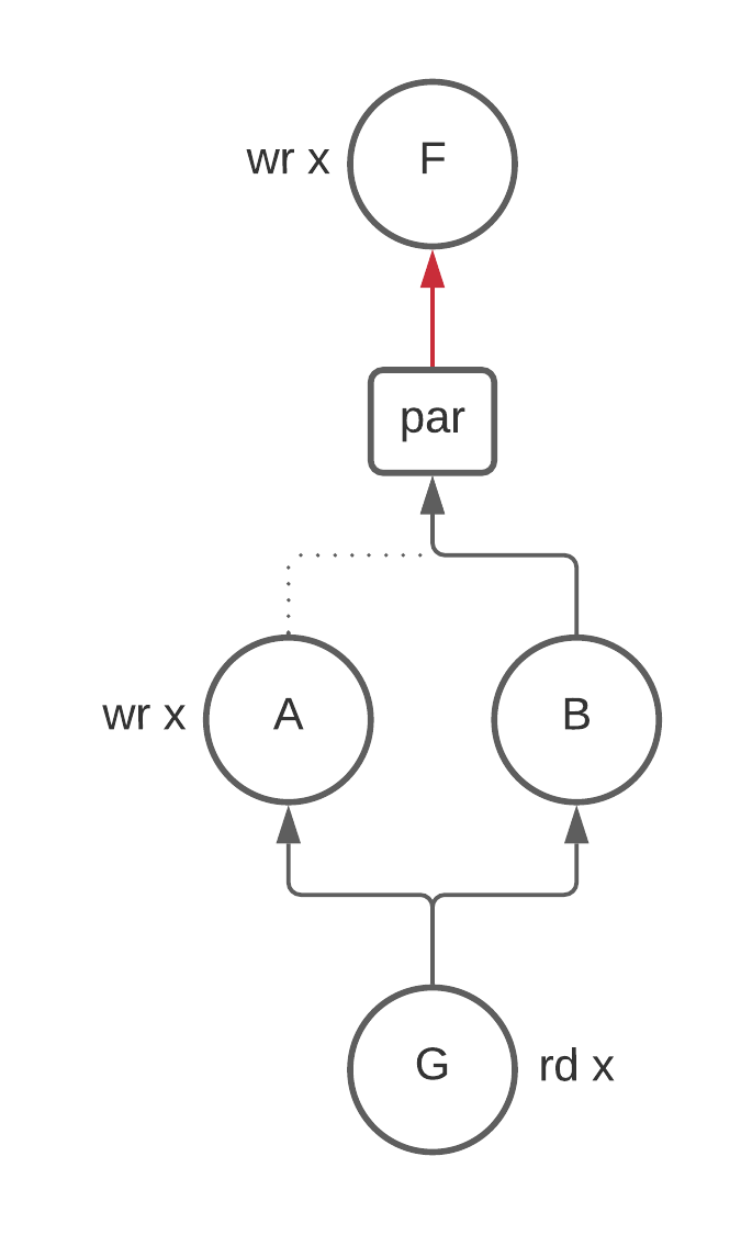
This is wrong because B doesn't kill x and so x is alive coming into B. The union preserves this information and results in x being alive above par.

Taking the set intersection is not quite right here either. Consider adding another group C that reads from x.

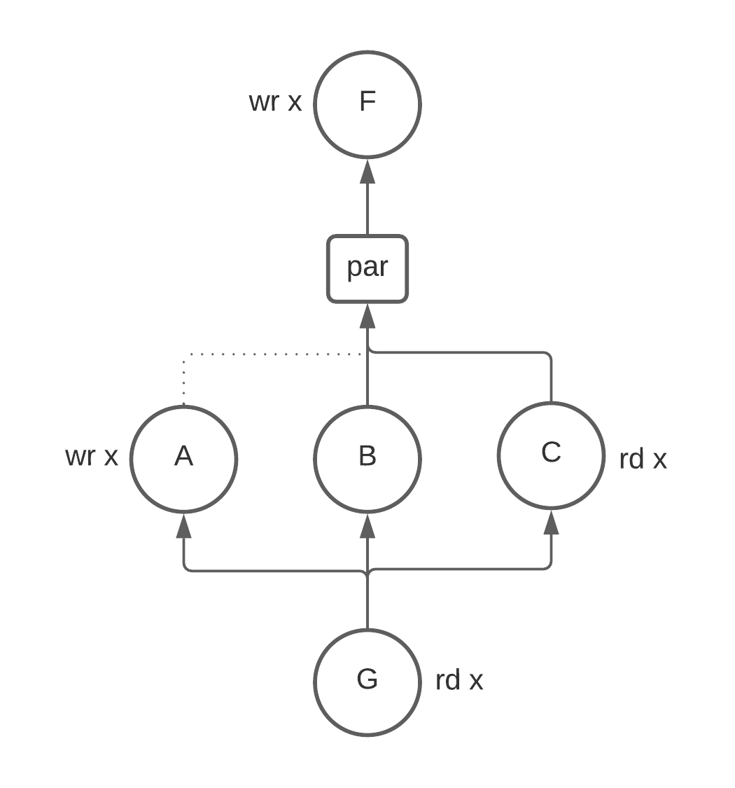
We have no information about how this read is ordered with the write to x in A so we have to assume that x is alive above par. If we take the intersection here:

  live(A) & live(B) & live(C)
= {} & {x} & {x}
= {}

We get the wrong answer. More generally, we can see that union clobbers any writes and intersection clobbers any reads that happen in the par.

The solution to this problem is solved by passing the gen and kill sets along with the live sets. Then par can set its output to be

(union(live(children)) - union(kill(children))) | union(gen(children))

The final tricky bit is thinking about how information flows between siblings in a par statement. Consider again the picture above with three nodes: A, B, and C. Should x be live at B? For liveness it turns out to be yes, but bare with me for a second for a thought experiment and consider the case where we have the guarantee that statements running in parallel can not interact with each other. This lets us reorder statements in some cases. Then there seems to be an information trade-off for how to define the liveness of x at B:

• You could say that x is dead at B because it doesn't see any previous writes to x and doesn't read from x. This implies that you could potentially replace writes to other registers with x. However, this by itself would cause x to be written to twice in parallel. You would have to reorder B to run before A. The takeaway here is that calling x dead at B gives the register reuse pass more information to work with. To compute this information B needs the gens and kills from all of its siblings (for the same reason that par) needed it. This is not particularly hard to implement, but it's worthy of noting.
• If you say that x is live at B, then you can never rewrite B to use x instead of some other register, but you also don't have to worry about reordering statements in a par.

Leaving thought experiment land, in our case we can never reorder statements in a par because siblings may interact with each other in arbitrary ways. For this reason, we must say that x is live at B. However, it's not immediately clear to me that this will be true of all dataflow analyses. That's why I set this thought experiment down in writing.

Equivalence to worklist algorithm

In the normal worklist algorithm, we add a statement back to the worklist when its predecessor has changed.

The intuition for why this algorithm is equivalent to worklist algorithm is that because the only entry into the children for each parent control statement is the parent control statement itself. The only way that a child statement would need to be recomputed is if the inputs to the parent need to be recomputed. Anything above the parent in the tree will take care of this re-computation.

Debugging

Calyx programs can provide wrong answers for two reasons:

1. The program implements the wrong algorithm, i.e., it has a logical bug.
2. The Calyx compiler incorrectly compiles the program, i.e., there is a compilation bug.

First make sure that the program generates the correct values with the Calyx Interpreter. If it produces the wrong values, your Calyx implementation of the algorithm is incorrect. You can use the Calyx Debugger to debug these problems.

If the interpreter produces the right values, try a different Verilog backed. We support both Verilator and Icarus Verilog. If both produce the wrong answer and the interpreter produces the right answer then you likely have a compilation bug on your hands. Use the debugging tips to narrow down the pass that causes the error.

Cider: The Calyx Interpreter and Debugger

Cider is a prototype debugging tool which exposes a gdb-like interface for debugging Calyx programs.

Getting Started

If you are using fud2, getting started with the debugger is easy. It requires no extra setup beyond the initial fud2 directory configuration.

Assuming you are trying to debug a program called my_program.futil with data file my_program.futil.data, invoke the debugger with the following command:

fud2 my_program.futil --to cider-debug -s sim.data=my_program.futil.data

This will open the target program in the interactive debugger.

Advancing Program execution

step

The simplest way to advance the program is via the step command which causes time to advance by a clock tick. It also has a shortcode: s.

 > step
 > s

The above snippet advances the program by two steps.

step-over

Another way to advance the program is via the step-over command. Unlike the step command, this command requires a second argument which is the name of the group to advance over. The step-over command then advances the program until the given group is no longer running.

If you want to use the command to advance the program past a group group_1, do the following:

 > step-over group_1

Note that the step-over command will do nothing if the given group is not running.

 > step-over other_group
 Group is not running
 >

continue

Finally, the continue command will run the program until either a breakpoint is hit or the program terminates. This command is used in conjunction with breakpoints and watchpoints to provide more targeted inspection. It may also be accessed with the shortcode c.

 > continue
Main component has finished executing. Debugger is now in inspection mode.

Breakpoints

Cider supports breakpoints on group definitions. This helps focus attention on suspect portions of the code.

Setting a breakpoint

Breakpoints may be set on the main component by simple specifying the group of interest.

 > break group_1

This is identical to

 > break main::group_1

For sub-components, the name of the sub-component must be included with the double colon separating the group name. To break on the do_mul group inside the pow sub-component:

 > break pow::do_mul

Managing breakpoints

To see a list of breakpoints:

 > info break

or

 > ib

This produces output like this:

 > ib
     Current breakpoints:
    1.  main::group_1  enabled
    2.  pow::do_mul enabled

All breakpoints have a number associated with them and they may be managed with this number or the group name.

To enable or disable a breakpoint:

 > disable group_1 2
 > enable 1 pow::do_mul

Note that this is equivalent to:

 > disable group_1
 > disable 2
 > enable 1
 > enable pow::do_mul

To delete a breakpoint:

 > delete 1
 > del pow::do_mul

Deleted breakpoints will be entirely removed while disabled breakpoints will remain until they are either enabled again or subsequently deleted. Disabled breakpoints will not cause program execution to halt when continue-ing.

Inspecting State

display

The display command dumps the full state of the main component without formatting. Use the print and print-state commands for targeted inspection with formatting.

Formatting codes

Cider supports several different formatting codes which do the hard work of interpreting the data in human readable ways.

print and print-state

These commands allow inspecting instance state with optional formatting. Note that this is different from breakpoints which operate on definitions. For example to print the ports of the std_mul instance named mul in the pow instance pow_1 attached to the main component:

 > print main.pow_1.mul

as with breakpoints, the leading main may be elided:

 > print pow_1.mul

This will print all the ports attached to this multiplier instance with binary formatting.

Formatting codes may be supplied as the first argument.

 > print \u pow_1.mul

The print may also target specific ports on cells, rather than just the cell itself. To see only the output of the multiplier (with unsigned formatting):

 > print \u pow_1.mul.out

The print-state command works in the same way as the print command, except it displays the internal state of a cell, rather than port values. As such, it can only target cells and only those with some internal state, such as registers or memories. For example, if the main component has a memory named out_mem its contents may be viewed via:

 > print-state main.out_mem

or just

 > print-state out_mem

As with print, print-state supports formatting codes as an optional first argument. So to view the contents of out_mem with a signed interpretation:

 > print-state \s out_mem

Watchpoints

Watchpoints are like breakpoints but rather than stop the execution when they are passed, they instead print out some information. Like breakpoints, they are set on group definitions, such as main::group_1 or pow::do_mul

Setting watchpoints

The general form of watchpoints looks like

watch [POSITION] GROUP with PRINT-COMMAND

where:

• GROUP is the group definition to be watched
• PRINT-COMMAND is a full print or print-state command to be run by the watchpoint

The optional POSITION argument may either be before or after. This specifies whether the watchpoint should run when the group first becomes active (before) or when the group finishes running (after). This defaults to before if not set.

Managing watchpoints

Watchpoint management is similar to breakpoints. However there may be multiple watchpoints for a single group definition, so deleting watchpoints via the group name will delete all the watchpoints associated with the group. Watchpoints do not currently have an enable/disable state.

To view all the watchpoint definitions:

 > info watch

...

 > iw

To delete watchpoints:

 > delete-watch 1
 > del-watch main::group_1

Viewing the program counter

There where command (alias pc) displays the currently running portion of the control tree including active subcomponents. This can be used to more easily determine the currently active portion of the design as well as visualize how much of the execution is occurring in parallel at any given point.

Exiting the debugger

Use help to see all commands. Use exit to exit the debugger.

Debugging Compilation Bugs

These tips are directed towards compilation bugs. Before trying these, make sure your program produces the correct values with the Calyx Interpreter.

Disabling Optimizations

The first step is disabling optimization passes and running the bare bones compilation pipeline.

To disable the passes, add the flag -p no-opt to compiler invocation:

1. For the compiler: calyx <filename> -p no-opt.
2. For fud: fud ... -s calyx.flags " -p no-opt".

If the output is still incorrect then one of the core compilation passes is incorrect. Our best bet at this point is to reduce the test file such that the output from the interpreter and the Calyx compiler still disagree and report the bug. We can use the waveform debugging to figure out which part of the compilation pipeline generates the incorrect result.

If the execution generates the right result, then one of the optimizations passes is incorrect. To identify which optimization pass is wrong, add back individual passes and see when the execution fails. The calyx/src/default_passes.rs file defines the compilation pipeline. Start by incrementally adding passes to this flag invocation:

-p validate -p simplify-with-control -p <PASS 1> ... -p <PASS N> -p compile -p lower

Reducing Test Files

It is often possible to reduce the size of the example program that is generating incorrect results. In order to perform a reduction, we need to run the program twice, once with a "golden workflow" that we trust to generate the right result and once with the buggy workflow.

Inlining (Optional)

It is useful to inline all the code into the main component so that we can focus our energy on reducing one control program. This can be done by passing the following flags to the compiler:

-p well-formed -p inline -x inline:always -p post-opt

The -x inline:always flag tells the inlining pass to attempt to inline all components into one. If this command fails, we can just work with the original program and reduce control programs for each component.

Reducing

At a high-level, we want to do the following:

1. Delete some part of the control program
2. See if the error still occurs
3. If it doesn't, delete a smaller part of the control program
4. Otherwise, continue deleting more parts of the control program

When deleting parts of the control program, the compiler may complain that certain groups are no longer being used. In this case, run the -p dead-group-removal pass before any other pass runs.

Next, if we've identified the problem to be in one of the Calyx passes, the "golden workflow" is running the program without the pass while the buggy workflow is running the program with the pass enabled. This case is so common that we've written a script that can run programs with different set of flags to the Calyx compiler and show the difference in the outputs after simulation.

The script is invoked as:

tools/flag-compare.sh <calyx program> <data>

By default, the script will try to run the programs by simulating them through Verilator by providing fud with the target --to dat. If you'd like to use the Calyx Interpreter instead, run the following command:

tools/flag-compare.sh <calyx program> <data> interpreter-out

Reducing Calyx Programs

The best way to reduce Calyx program deleting group enables from the control program and seeing if the generated program still generates the wrong output. While doing this, make sure that you're not deleting an update to a loop variable which might cause infinite loops.

By default, the compiler will complain if the program contains a group that is not used in the control program which can get in the way of minimizing programs. To get around this, run the dead-group-removal pass before the validation passes:

calyx -p dead-group-removal -p validate ...

Reducing Dahlia Programs

If you're working with Dahlia programs, it is also possible to reduce the program with the script since it simply uses fud to run the program with the simulator. As with Calyx reduction, try deleting parts of the program and seeing if the flag configurations for the Calyx program still generate different outputs.

Waveform Debugging

Waveform debugging is the final way of debugging Calyx programs. A waveform captures the value of every port at every clock cycle and can be viewed using a wave viewer program like GTKWave or WaveTrace to look at the wave form. Because of this level of granularity, it generates a lot of information. To make the information a little more digestible, we can use information generated by Calyx during compilation.

For waveform debugging, we recommend disabling the optimization passes and static timing compilation (unless you're debugging these passes). In this debugging strategy, we'll do the following:

1. Dump out the control FSM for the program we're debugging.
2. Find the FSM states that enable the particular groups that might be misbehaving.
3. Open the waveform viewer and find clock cycles where the FSM takes the corresponding values and identify other signals that we care about.

Consider the control section from examples/futil/dot-product.futil:

    seq {
      let0;
      while le0.out with cond0 {
        seq {
          par {
            upd0;
            upd1;
          }
          let1;
          let2;
          upd2;
          upd3;
        }
      }
    }

Suppose that we want to make sure that let0 is correctly performing its computation. We can generate the control FSM for the program using:

  calyx <filename> -p top-down-cc

This generates a Calyx program with several new groups. We want to look for groups with the prefix tdcc which look something like this:

group tdcc {
  let0[go] = !let0[done] & fsm.out == 4'd0 ? 1'd1;
  cs_wh.in = fsm.out == 4'd1 ? le0.out;
  cs_wh.write_en = fsm.out == 4'd1 ? 1'd1;
  cond0[go] = fsm.out == 4'd1 ? 1'd1;
  par[go] = !par[done] & cs_wh.out & fsm.out == 4'd2 ? 1'd1;
  let1[go] = !let1[done] & cs_wh.out & fsm.out == 4'd3 ? 1'd1;
  let2[go] = !let2[done] & cs_wh.out & fsm.out == 4'd4 ? 1'd1;
  upd2[go] = !upd2[done] & cs_wh.out & fsm.out == 4'd5 ? 1'd1;
  upd3[go] = !upd3[done] & cs_wh.out & fsm.out == 4'd6 ? 1'd1;
  ...
}

The assignments to let0[go] indicate what conditions make the let0 group execute. In this program, we have:

let0[go] = !let0[done] & fsm.out == 4'd0 ? 1'd1;

Which states that let0 will be active when the state of the fsm register is 0 along with some other conditions. The remainder of the group defines how the state in the fsm variable changes:

  ...
  fsm.in = fsm.out == 4'd0 & let0[done] ? 4'd1;
  fsm.write_en = fsm.out == 4'd0 & let0[done] ? 1'd1;
  fsm.in = fsm.out == 4'd1 & cond0[done] ? 4'd2;
  fsm.write_en = fsm.out == 4'd1 & cond0[done] ? 1'd1;
  ...

For example, we can see that when the value of the FSM is 0 and let0[done] becomes high, the FSM will take the value 1.

Once we have this information, we can open the VCD file and look at points when the fsm register has the value 1 and check to see if the assignments in let0 activated in the way we expected.

Contributing to Calyx

Github Workflow

The current home of the Calyx repo can be found here. As with many large projects, we protect the main branch of the repo so that updates can only be made via pull requests. So the development cycle tends to look like:

checkout main -> develop code -> open PR -> revise -> merge PR

For legibility of commits, we squash all commits in a PR down to a single commit and merge the composite commit to the main branch. This helps keep the commit count of the main branch lower than it would otherwise be; however, it can make using commands like git bisect more challenging for large branches. For that reason we tend to recommend more frequent PRs to avoid large deltas.

Once your PR has been merged, be sure to check out the updated main branch for future changes. If you branch off the merged branch or continue with it, there will be extensive merge conflicts due to the squash and merge tactic. For this reason we always recommend creating branches off of the main branch if you intend to have them merged into it.

Local Development

Once you've setup a local installation for contributing, you can setup git hooks with /bin/sh setup_hooks.sh.

CI Behavior

The CI runs a number of tests including ensuring that Rust and Python code has been formatted. For Python we use the Black formatter and for Rust we use the standard cargo fmt.

For Rust further linting is done via clippy to ensure that there are no warnings. In situations where warnings are expected, such as code that is only part way through development, you can opt to add #[allow] annotations within Rust to suppress the lint.

If changes are made to the Dockerfile then the CI will automatically rebuild the Docker image and run your tests on it.

Emitting Calyx from Python

The calyx builder library provisions an embedded domain-specific language (eDSL) that can be used to generate Calyx code. The DSL is embedded in Python.

Installation

To install the library, run the following from the repository root. The command requires flit, which you can install with pip install flit.

cd calyx-py && flit install -s

Hello, Calyx World!

We will start by using the calyx library to generate a simple Calyx program. Glance through the Python code below, which is also available at helloworld.py.

import calyx.builder as cb
import os


def insert_adder_component(prog):
    comp = prog.component("adder")

    val1 = comp.input("val1", 32)
    val2 = comp.input("val2", 32)
    comp.output("out", 32)

    sum = comp.reg(32)
    add = comp.add(32)

    with comp.group("compute_sum") as compute_sum:
        add.left = val1
        add.right = val2
        sum.write_en = cb.HI
        sum.in_ = add.out
        compute_sum.done = sum.done

    with comp.continuous:
        comp.this().out = sum.out

    comp.control += compute_sum


if __name__ == "__main__":
    prog = cb.Builder(fileinfo_base_path=os.path.dirname(os.path.realpath(__file__)))
    insert_adder_component(prog)
    prog.program.emit()

Running this Python code, with

python calyx-py/test/helloworld.py

will generate the following Calyx code. As you may have inferred, we are have simply created a 32-bit adder in a contrived manner.

import "primitives/core.futil";
import "primitives/binary_operators.futil";
component adder<"pos"={0}>(val1: 32, val2: 32) -> (out: 32) {
  cells {
    @pos{1} reg_1 = std_reg(32);
    @pos{2} add_2 = std_add(32);
  }
  wires {
    group compute_sum<"pos"={3}> {
      add_2.left = val1;
      add_2.right = val2;
      reg_1.write_en = 1'd1;
      reg_1.in = add_2.out;
      compute_sum[done] = reg_1.done;
    }
    out = reg_1.out;
  }
  control {
    @pos{4} compute_sum;
  }
}

sourceinfo #{
FILES 
  0: helloworld.py
POSITIONS 
  0: 0 6
  1: 0 12
  2: 0 13
  3: 0 15
  4: 0 25
}#

Walkthrough

So far, it does not look like using our eDSL has bought us much. We have essentially written Calyx, line by line, in Python. However, it is useful to go through the process of generating a simple program to understand the syntax and semantics of the builder library.

For each item discussed below, we encourage you to refer to both the Python code and the generated Calyx code.

We add the component adder to our program with the following line:

    comp = prog.component("adder")

We then specify the names and bitwidths of any ports that we want the component to have.

    val1 = comp.input("val1", 32)
    val2 = comp.input("val2", 32)
    comp.output("out", 32)

We also add two cells to the component: a 32-bit adder and a 32-bit register.

    sum = comp.reg(32)
    add = comp.add(32)

The heart of the component is a group of assignments. We begin the group with:

    with comp.group("compute_sum") as compute_sum:

We know that we have instantiated a std_add cell, and that such a cell has input ports left and right. We need to assign values to these ports, and we do so using straightforward dot-notated access. The values val1 and val2 exactly the inputs of the component.

        add.left = val1
        add.right = val2

Now we would like to write the output of the adder to a register. We know that registers have input ports write_en and in. We assert the high signal on write_en with:

        sum.write_en = cb.HI

We specify the value to be written to the register with:

        sum.in_ = add.out

Although the port is named in, we must use in_ to avoid a clash with Python's in keyword. Observe that we have used dot-notated access to both read the out port of the adder and write to the in port of the register.

Since compute_sum is a group of assignments, we must specify when it is done. We do this with:

        compute_sum.done = sum.done

That is, the group is done when the register we are writing into asserts its done signal.

In order to add a continuous assignment to our program, we use the construct with {component}.continuous:. To access the ports of a component while defining it, we use the this() method.

    with comp.continuous:
        comp.this().out = sum.out

That is, we want this component's out port to be continuously assigned the value of the sum's out port.

Finally, we construct the control portion of this Calyx program:

    comp.control += compute_sum

We have some boilerplate code that creates an instance of the builder, adds to it the component that we have just studied, and emits Calyx code.

if __name__ == "__main__":
    prog = cb.Builder()
    insert_adder_component(prog)
    prog.program.emit()

Further, the builder library is able to infer which Calyx libraries are needed in order to support the generated Calyx code, and adds the necessary import directives to the generated code.

Further Reading

The builder library walkthrough contains a detailed description of the constructs available in the builder library.

Other examples using the builder can also be found in the calyx-py test directory. All of our frontends were also written using this library, in case you'd like even more examples!

Builder Library Walkthrough

This is an extended walkthough of all the features of the Calyx builder library. The builder library is an embedded DSL, embedded in Python, that allows users to generate Calyx code programmatically.

This page seeks to demonstrate all the features of the builder library. For a quick start, we refer you to the hello world example.

We will make repeated references to the example program walkthrough.py, which emits the Calyx codewalkthrough.expect when run. We recommend that you refer to these files as you work through this document.

Components

We add a component to our program as follows:

    comp = prog.component("adder")

Ports of Components

We specify the names and bitwidths of any ports that we want a component to have as follows:

    val1 = comp.input("val1", 32)
    val2 = comp.input("val2", 32)
    comp.output("out", 32)

Observe that we have saved handles to the input ports by assigning them to Python variables, but have not done the same with the output port. We will show shortly how to create a handle to a port after its definition.

It is also possible to create ports that have attributes. Attributes can either be described as a string or a (string, value) tuple. A string such as "data", which will create an @data attribute. A (string, value) tuple such as ("done", 1) will create an @done(1) attribute.

    comp.output("out_2", 1, ["data"])
    comp.output("out_3", 1, ["data", ("done", 1)])

Cells

We add cells to the component as follows. The standard cells are all supported. Bitwidths must be passed as arguments, while names are optional.

    sum = comp.reg(32)
    add = comp.add(32)

The adder defined above is unsigned; we would define a signed variant as:

    add = comp.add(32, signed=True)

Groups

We begin a group with:

    with comp.group("compute_sum") as compute_sum:

We add wires within a group by staying within the indentation of the with block.

Combinational groups are written similarly, but with comb_group instead of group:

    with comp.comb_group("update_register") as update_register:

Static groups are written with static_group, and must specify a latency. The group below will take 3 cycles to execute:

    with comp.static_group("multiply", 3) as compute_sum:

Ports of Cells

We access ports of cells using dot notation.

        add.left = val1
        add.right = val2

Special Case: in_

We specify the value to be written to a register with:

        sum.in_ = add.out

Although the Calyx port is named in, we must write in_ in the eDSL to avoid a clash with Python's in keyword.

HI and LO Signals

The builder library provides shorthand for high and low signals.

        sum.write_en = cb.HI

There is a corresponding LO signal. These are just one-bit values 1 and 0, respectively.

Group done Signals

Groups that are not combinational must raise a done signal.

        compute_sum.done = sum.done

Accessing Output Ports of Components

We can create a handle to a port after its definition.

    with comp.continuous:
        comp.this().out = sum.out

That is, comp.this().out is a handle to the port named "out" on the component whose handle is comp.

Accessing ports in this way may feel silly, since we have already shown that we can save handles to ports by assigning them to Python variables. This does work for input ports, but not for output ports.

Say we had saved a handle to the output port of the adder component:

out = comp.output("out", 32)

Now say we wanted to say that the output port gets the value of the sum's output port:

out = sum.out

Python will get in our way because it will think that out is a variable that is written to (twice!) but never read from.

To avoid this, we use the this() method to access the output ports of a component.

Continuous Assignments

Continuous assignments are added using with {component}.continuous:.

    with comp.continuous:
        comp.this().out = sum.out

Simple Control Program

A simple control program is added to the component as follows. This is just enabling the group that we have defined.

    comp.control += compute_sum

Binary Operation and Store

The library provides a shorthand for the common pattern of performing a binary operation and writing the result to a register.

    diff_group_1, _ = comp.sub_store_in_reg(val1, val2, diff)

Here diff is a handle to a register that we have defined earlier. This single line of Python adds lines to the cells and the wires sections of the Calyx code:

  cells {
    sub_1 = std_sub(32);
  }
  wires {
    group sub_1_group {
      sub_1.left = val1;
      sub_1.right = val2;
      diff.write_en = 1'd1;
      diff.in = sub_1.out;
      sub_1_group[done] = diff.done;
    }
  }

In Python, its return value is a handle to the group that it has created, and a handle to the register is has written to. In the line of Python above, we have saved the handle to the group (as diff_group_1) but have discarded the handle to the register using a _ variable name since we already have a handle to the register, diff.

This construct can also be called without passing a register, in which case it will create a register and return it. It is useful in that case to save the handle to the register.

Operation-Use

The library provides a shorthand for the common pattern of performing a binary operation and using the result combinationally.

    val2_lt_val1 = comp.lt_use(val2, val1)

This line of Python adds lines to the cells and the wires sections of the Calyx code:

cells {
    lt_3 = std_lt(32);
  }
  wires {
    comb group lt_3_group {
      lt_3.left = val2;
      lt_3.right = val1;
    }
  }

Note that the group is combinational, and so does not need a done signal.

The value returned by this function, which we have saved above as val2_lt_val1 is in fact a tuple of handles: a handle to the group that it has created and a handle to the cell that that group uses. We shall see shortly how to use this tuple.

Complex Control: par, seq, if

Let us work through a slightly more complex control program.

    comp.control += cb.par(
        [
            val1_ge_val2,
            cb.if_(ge_reg.out, diff_group_1, diff_group_2),
        ],
        cb.if_with(val2_lt_val1, diff_group_2, diff_group_1),
    )

We run control operators in sequence by making them elements of a list. This is why the group val1_ge_val2 runs before the if check written on the next line.

We run control operators in parallel by passing them to the par function.

The if_ function (named with the underscore to avoid clashing with Python's if keyword) is a straightforward if check. It takes a condition, a body, and an optional else body.

The if_with function is a slightly more complex if check. It takes a (cell, comb_group) tuple, a body, and an optional else body. It generates a combinational if check, of the form

if cell.out with comb_group ...

It is especially useful in concert with the Operation-Use construct, which returns exactly such a tuple of a cell and a group.

Multi-Component Designs

Using one component in another is straightforward.

We must first define the called component as a cell of the calling component, and then we can use the cell as usual.

Say we have a handle, diff_comp, to the component that we wish to call. Say also that we know that the component has input ports val1 and val2, and an output port out.

We can write:

    abs_diff = comp.cell("abs_diff", diff_comp)
    with comp.group("compute_diff") as diff_group:
        abs_diff.val1 = val1
        abs_diff.val2 = val2
        abs_diff.go = cb.HI
        mux.write_en = abs_diff.done
        mux.in_ = abs_diff.out
        diff_group.done = mux.done

Although the called component did not have explicit go and done ports, the builder library has added them for us. We use these ports to guide the execution of the group. We assert the go signal to the called component with diff_comp.go = HI, and then, by writing mux.write_en = abs_diff.done, we make the write to the register mux conditional on the done signal of the called component.

Memories

We can define memories in a component as follows:

    mem = comp.comb_mem_d1("mem", 32, 10, 32, is_ref=True)

This is a 1-D memory with ten 32-bit entries, each 32 bits wide. We have additionally declared that this memory will be passed to the component by reference. We shall see how shortly.

Miscellaneous Higher-Level Constructors

As patterns of use emerge, we can add further constructors to the builder library to support common use-cases. For example, we can add a constructor that increments a register by a constant value.

    incr_i = comp.incr(i)

That line of Python adds lines to the cells and the wires sections of the Calyx code:

  cells {
    i_incr = std_add(8);
  }
  wires {
    group i_incr_group {
      i_incr.left = i.out;
      i_incr.right = 8'd1;
      i.write_en = 1'd1;
      i.in = i_incr.out;
      i_incr_group[done] = i.done;
    }
  }

The Python return value, incr_i, is a handle to the group that performs the incrementing. The method defaults to incrementing by 1, but can be passed any value.

Guarded Assignments

Consider the group that multiplies the memory at the cell pointed to by register i by the value v.

    with comp.group("mul_at_position_i") as mul_at_position_i:
        mem.addr0 = i.out
        mul.left = mem.read_data
        mul.right = v
        mem.write_en = mul.done @ cb.HI
        mem.write_data = mul.out
        mul_at_position_i.done = mem.done

The first few lines are straightforward; we are setting the cell to be read from with addr0, reading from that cell and driving the value to the multiplier's left port, and setting the right port of the multiplier to the value v.

Now we wish to write the result to the memory at the cell pointed to by register i, but only once we know that the multiplier has finished its work. We do this with a guarded assignment, using the @ operator:

        mem.write_en = mul.done @ cb.HI

In Calyx, we would have written this guarded assignment with a question mark:

        mem.write_en = mul.done ? 1'd1;

We use the @ operator in the builder library to avoid clashing with Python's ternary operator.

Complex Control: while

The builder library supports while loops and also the higher-level while_with constructor.

    comp.control += cb.while_with(i_lt_10, [mul_at_position_i, incr_i])

Here i_lt_10 is a tuple of two handles, exactly as returned by the Operation-Use constructor. The while_with constructor takes this tuple and a body.

External Memories

We can define external memories in a component, typically the main component, as follows:

    mymem = comp.comb_mem_d1("mymem", 32, 10, 32, is_external=True)

Invoking Components

We can invoke components as follows:

        cb.invoke(map, ref_mem=mymem, in_v=cb.const(32, 42))

That is, we have a Python-level handle to some component map that has one memory called mem that it expects to be passed by reference, and one input port called v. We must prepend ref_ to the names of any memories, and in_ to the names of any input ports.

Building the Program

Finally, we build the program.

def build():
    prog = cb.Builder(fileinfo_base_path=os.path.dirname(os.path.realpath(__file__)))
    insert_adder_component(prog)
    diff_comp = insert_abs_diff_component(prog)
    insert_mux_component(prog, diff_comp)
    map_comp = insert_map_component(prog)
    insert_main_component(prog, map_comp)
    return prog.program

Note that all of our component-inserting helpers have been returning the components that they have created. This is so that we can build complex programs where components either call each other as cells or invoke each other.

This is why we save a Python-level handle to the diff_comp component that we have defined, and then pass it to the insert_mux_component function. As we have seen, the mux uses diff_comp as a cell.

We also save a Python-level handle to the map component that we have defined, and then pass it to the insert_main_component function. As we have seen, map is invoked by main.

Emitting the Program

Finally, we emit Calyx.

if __name__ == "__main__":
    build().emit()

Retrieving Items by Name

In the discussion so far, we have guided you towards a pattern of defining an item (a cell, a group, a component, etc.) and then saving a handle to it as a Python variable. This is a good pattern to follow, but it is not the only one.

To reference a component without an existing handle to it, use the Builder().get_component() method.

prog.component("my_component")
# a few lines later
my_component = prog.get_component("my_component")

To access the input and output ports of a component within the definition of a component, use the syntax my_component.this().port.

def add_my_component(prog):
    my_component = prog.component("my_component")
    my_component.output("my_output", 32)

    with my_component.group("my_group"):
        my_component.this().my_output = const(32, 1)

In order to reference a cell without a handle use the Builder().get_cell() method.

my_component.reg("my_reg", 32)
# a few lines later
my_reg = prog.get_cell("my_reg")

A group can be retrieved with the Builder().get_group() method. It's possible to retrieve combinational groups as well as regular groups with this method.

with my_component.group("my_group"):
    # group definition here
# a few lines later
my_group = prog.get_group("my_group")

Defining Component Attributes

Components can be given attributes. Similar to ports, just specify the name of the attribute and its value. Note that attribute(name, value) does not return a handle to the attribute.

my_component.attribute("my_attribute", 1)

Will create a component that looks like:

component my_component<"my_attribute"=1>(...) -> (...) {

Importing Calyx Libraries

The builder library imports necessary Calyx libraries automatically. However, it is possible to import additional libraries manually.

prog = cb.Builder()
prog.import_("primitives/binary_operators.futil")

Explictly Stating Widths

Usually, the builder library can automatically infer the widths of constants. In cases where it cannot, it will complain at Python compilation. Use the const(width, value) expression to explicitly state the width of a constant.

my_cell.my_port = const(32, 1)

Components with Known Latency

You can declare a component to be static by stating its latency when declaring it. For instance, our contrived adder from above could be declared as static with a latency of one cycle as follows:

comp = prog.component("adder", latency=1)

As a reminder, the regular version is just:

comp = prog.component("adder")

Building a Frontend for Calyx

This tutorial assumes that you have already worked through the Calyx tutorial. You won't get very much out of it by itself!

In the Calyx tutorial you wrote Calyx code by hand. This is (probably) a good way to build character, but it's no way to live. Indeed, Calyx was designed to be a compiler IL, and not a human-facing language.

In this tutorial, we're going to learn all about this by building a DSL-to-hardware compiler for a toy language that we wish to accelerate. We will compile the DSL to Calyx, and then let Calyx take us to hardware.

MrXL Overview

Meet MrXL, our toy DSL. MrXL lets you define arrays and registers and then perform map and reduce operations.

Example: sum of squares

Here's a MrXL program that squares and then sums the values of an input array:

input avec: int[4]
output sos: int
squares := map 1 (a <- avec) { a * a }
sos := reduce 1 (acc, i <- squares) 0 { acc + i }

This short program shows off all of MrXL's features, so let's pick it apart line by line:

1. We specify an array, avec, which will have four integers. The input keyword means that an external harness will populate the array.
2. We specify sos, a register. The output keyword means that we will populate sos in our program.
3. The map operation gets the values of avec and raises each to the second power. We stash the result in a new array, squares. The number 1 denotes a parallelism factor of 1, meaning that the operation is performed sequentially. We will improve this shortly.
4. The reduce operation walks over squares and accumulates the result into a register. The parallelism factor is again 1.

Running our example

Installing MrXL

If you are going through this tutorial in the Docker container, you can skip these installation steps and jump to Running MrXL just below.

First, install the builder library by typing the following command from the repository root:

cd calyx-py && flit install -s && cd -

Next, install the mrxl binary:

cd frontends/mrxl && flit install -s && cd -

Register the mrxl binary with fud:

fud register mrxl -p frontends/mrxl/fud/mrxl.py

Now, running fud check should report that the mrxl binary is correctly installed.

Running MrXL

Run:

mrxl frontends/mrxl/test/sos.mrxl --data frontends/mrxl/test/sos.mrxl.data --interpret

Why 42? Because we populated avec with:

{
  "avec": [
    0,
    1,
    4,
    5
  ]
}

and \( 0^2 + 1^2 + 4^2 + 5^2 = 42 \).

Compiling our example into Calyx

Above, we merely interpreted MrXL code in software using a simple, pre-written interpreter implemented in Python. Our goal in this tutorial is to build a compiler from MrXL to hardware by translating it to the Calyx IL. The Calyx IL code generated by compiling this program looks more like:

import "primitives/core.futil";
import "primitives/binary_operators.futil";
component main() -> () {
  cells {
    @external avec_b0 = comb_mem_d1(32, 4, 32);
    @external sos = comb_mem_d1(32, 1, 32);
    sos_reg = std_reg(32);
    squares_b0 = comb_mem_d1(32, 4, 32);
    idx_b0_0 = std_reg(32);
    incr_b0_0 = std_add(32);
    lt_b0_0 = std_lt(32);
    mul_b0_0 = std_mult_pipe(32);
    idx1 = std_reg(32);
    incr_1 = std_add(32);
    lt_1 = std_lt(32);
    add_1 = std_add(32);
  }
  wires {
    group sos_reg2mem {
      sos.addr0 = 32'd0;
      sos.write_data = sos_reg.out;
      sos.write_en = 1'd1;
      sos_reg2mem[done] = sos.done;
    }
    group incr_idx_b0_0 {
      incr_b0_0.left = idx_b0_0.out;
      incr_b0_0.right = 32'd1;
      idx_b0_0.in = incr_b0_0.out;
      idx_b0_0.write_en = 1'd1;
      incr_idx_b0_0[done] = idx_b0_0.done;
    }
    comb group cond_b0_0 {
      lt_b0_0.left = idx_b0_0.out;
      lt_b0_0.right = 32'd4;
    }
    group eval_body_b0_0 {
      avec_b0.addr0 = idx_b0_0.out;
      mul_b0_0.left = avec_b0.read_data;
      mul_b0_0.right = avec_b0.read_data;
      squares_b0.addr0 = idx_b0_0.out;
      squares_b0.write_data = mul_b0_0.out;
      mul_b0_0.go = 1'd1;
      squares_b0.write_en = mul_b0_0.done;
      eval_body_b0_0[done] = squares_b0.done;
    }
    group init_idx_1 {
      idx1.in = 32'd0;
      idx1.write_en = 1'd1;
      init_idx_1[done] = idx1.done;
    }
    group incr_idx_1 {
      incr_1.left = idx1.out;
      incr_1.right = 32'd1;
      idx1.in = incr_1.out;
      idx1.write_en = 1'd1;
      incr_idx_1[done] = idx1.done;
    }
    comb group cond_1 {
      lt_1.left = idx1.out;
      lt_1.right = 32'd4;
    }
    group init_1 {
      sos_reg.in = 32'd0;
      sos_reg.write_en = 1'd1;
      init_1[done] = sos_reg.done;
    }
    group reduce1 {
      squares_b0.addr0 = idx1.out;
      add_1.left = sos_reg.out;
      add_1.right = squares_b0.read_data;
      sos_reg.in = add_1.out;
      sos_reg.write_en = 1'd1;
      reduce1[done] = sos_reg.done;
    }
  }
  control {
    seq {
      par {
        while lt_b0_0.out with cond_b0_0 {
          seq {
            eval_body_b0_0;
            incr_idx_b0_0;
          }
        }
      }
      seq {
        par {
          init_1;
          init_idx_1;
        }
        while lt_1.out with cond_1 {
          seq {
            reduce1;
            incr_idx_1;
          }
        }
      }
      par {
        sos_reg2mem;
      }
    }
  }
}

Generate it for yourself! Run:

mrxl frontends/mrxl/test/sos.mrxl

Simulating our example with Verilog

Finally, let us go the whole hog: we compile our MrXL program to Calyx, compile it to Verilog, then simulate it using Verilator.

Run:

fud e --from mrxl frontends/mrxl/test/sos.mrxl --to dat --through verilog -s mrxl.data frontends/mrxl/test/sos.mrxl.data

The above command takes a MrXL program, sos.mrxl, and generates results with Verilator using the MrXL data file sos.mrxl.data.

Compiling MrXL into Calyx

Calyx is an infrastructure for designing domain-specific languages (DSL) which can generate efficient hardware. The rest of the tutorial will show you how to implement such a DSL by studying the MrXL-to-Calyx compiler, written in Python.

We have placed a few simplifying restrictions on MrXL programs:

1. Every array in a MrXL program has the same length.
2. Every integer in our generated hardware is 32 bits long.
3. The bodies of map and reduce operations must be binary + or * operations involving array elements or integers.
4. If repeated map/reduce operations are performed on the same array, each of those operations must have the same parallelism factor.
5. All reduce operations must be performed sequentially, i.e., with parallelism factor 1.

These restrictions can be lifted or relaxed via commensurate changes to the compiler.

The compilation process breaks into two steps:

1. Parsing MrXL into a representation we can process in Python.
2. Generating Calyx code.

Parsing MrXL into an AST

To start, we'll parse the MrXL program into a Python AST representation. We choose to represent AST nodes with Python dataclasses. A program is a sequence of array/register declarations followed by computation statements:

@dataclass
class Prog:
    """A MrXL program."""
    decls: List[Decl]  # Memory declarations
    stmts: List[Stmt]  # Map and reduce statements

Decl nodes correspond to array declarations such as input avec: int[4]. They carry information about whether the array is an input or output, the array's name, and the type of the array's elements:

@dataclass
class Decl:
    """Declaration of a memory."""
    input: bool  # If `False`, this is an `output`.
    name: str
    type: Type

Stmt nodes represent statements such as sos := reduce 1 (acc, i <- squares) 0 { acc + i }. They contain further nested nodes representing the function-header and -body, and the type of operation:

@dataclass
class Stmt:
    """A statement in the program."""
    dst: str
    operation: Union[Map, Reduce]

We elide further details, but point you to the AST, which defines all the nodes we need to represent a MrXL program.

Generating Calyx code

As you know, the skeleton of a Calyx program has three sections:

component main() -> {
  cells {}
  wires {}
  control {}
}

The cells section instantiates hardware units like adders, memories and registers. The wires section contains groups that connect hardware instances to perform some logical task (e.g, incrementing a register). Finally, the control section schedules the execution of groups using control operators such as seq, par, and while.

We perform syntax-directed compilation by walking over the nodes of the AST and generating cells, wires, and control operations.

An Embedded DSL that Generates Calyx

To make it easy to generate hardware, we'll use Calyx's builder module written in Python:

import calyx.builder as cb

prog = cb.Builder() # A Calyx program
main = prog.component("main") # Create a component named "main"

Decl nodes

Decl nodes instantiate new memories and registers. We need these to be instantiated in the cells section of our Calyx output. We use Calyx's std_reg and comb_mem_d1 primitives to represent registers and memories:

import "primitives/core.futil"; // Import standard library

component main() -> () {
  cells {
    // A memory with 4 32-bit elements. Indexed using a 6-bit value.
    avec = comb_mem_d1(32, 4, 6);
    // A register that contains a 32-bit value
    sos = std_reg(32);
  }
  ...
}

For each Decl node, we need to determine if we're instantiating a memory or a register, translate the node into a corresponding Calyx declaration, and place the declaration inside the cells section of our generated program.

If a memory is used in a parallel map or reduce, we might need to create different physical banks for it. We explain why below. We define a function to walk over the AST and compute the parallelism factor for each memory:

    # Collect banking factors.
    par_factor = compute_par_factors(prog.stmts)

Using this information, we can instantiate registers and memories for our inputs and outputs:

            for i in range(par):
                main.comb_mem_d1(
                    f"{name}_b{i}", 32, arr_size // par, 32, is_external=True
                )

The main.mem_d1 call is a function defined by the Calyx builder module to instantiate memories for a component. By setting is_external=True, we're indicating that a memory declaration is a part of the component's input-output interface.

Compiling map operations

For every map or reduce node, we need to generate Calyx code that iterates over an array, performs some kind of computation, and then stores the result of that computation. For map operations, we'll perform a computation on every element of an input array, and then store the answers in a result array. We can use Calyx's while loops to do this. At a high level, we want to generate the following pieces of hardware:

1. A register to store the current value of the loop index.
2. A comparator to check of the loop index is less than the array size.
3. An adder to increment the value of the index.
4. Whatever hardware is needed to implement the loop body computation.

We have implemented exactly this, and you have been using it thus far with the fud invocations that we have provided you.

However, it is time to get your hands dirty. We provide a stub implementation of map in gen_calyx.py:

def my_map_impl(
    comp: cb.ComponentBuilder,
    dest: str,
    stmt: ast.Map,
    arr_size: int,
    bank_factor: int,
    s_idx: int,
):
    """
    Returns a dictionary containing Calyx cells, wires and
    control needed to implement a `map` statement.
    See gen_stmt_impl for format of the dictionary.

    Generates these groups:
      - a group that implements the body of the `map` statement
      - a group that increments an index to access the `map` input array
      - a group that implements the loop condition, checking if the index
        has reached the end of the input array
    """
    # TODO: Implement map!
    return Empty()

You are invited to try implementing map yourself according to the outline given in the description by filling in the body of this function.

To run mrxl with my_map_impl instead of our implementation, pass the --my-map flag:

fud e --from mrxl test/sos.mrxl \
        --to dat --through verilog \
        -s mrxl.flags "--my-map "  \
        -s mrxl.data test/sos.mrxl.data

If you are feeling good about your implementation, skip to the next section! If you'd like to read through the details of our implementation – or build yours in tandem – continue on with the rest of this section.

Loop condition

We define a combinational group to perform the comparison idx < arr_size that uses an lt cell:

    group_name = f"cond_{suffix}"
    cell = f"lt_{suffix}"
    less_than = comp.cell(cell, Stdlib.op("lt", 32, signed=False))
    with comp.comb_group(group_name):
        less_than.left = idx.out
        less_than.right = arr_size

Index increment

The loop index increment is implemented using a group and an adder:

    group_name = f"incr_idx_{suffix}"
    adder = comp.add(32)
    with comp.group(group_name) as incr:
        adder.left = idx.out
        adder.right = 1
        idx.in_ = adder.out
        idx.write_en = 1
        incr.done = idx.done

We provide the index's previous value and the constant 1 to adder, and write the adder's output into the register (idx). Because we're performing a stateful update of the register, we must wait for the register to state that it has committed the write. We do this by setting the group's done condition to track the register's done signal.

Body computation

The final piece of the puzzle is the body's computation. The corresponding group indexes into the input memories:

        with comp.group(f"eval_body_{suffix}") as evl:
            # Index each array
            for bind in stmt.binds:
                # Map bindings have exactly one dest
                mem = comp.get_cell(f"{name2arr[bind.dst[0]]}")
                mem.addr0 = idx.out

Because the builder module is an embedded DSL, we can simply use Python's for loop to generate all the required assignments for indexing.

This code instantiates an adder or a multiplier depending on the computation needed using the expr_to_port helper function:

        if body.operation == "mul":
            operation = comp.cell(
                f"mul_{suffix}", Stdlib.op("mult_pipe", 32, signed=False)
            )
        else:
            operation = comp.add(32, f"add_{suffix}")

and writes the value from the operation into the output memory:

            out_mem = comp.get_cell(f"{dest}_b{bank}")
            out_mem.addr0 = idx.out
            out_mem.write_data = operation.out
            # Multipliers are sequential so we need to manipulate go/done signals
            if body.operation == "mul":
                operation.go = 1
                out_mem.write_en = operation.done
            else:
                out_mem.write_en = 1
            evl.done = out_mem.done

This final operation is complicated because we must account for whether we're using an adder or a multiplier. Adders are combinational–they produce their output immediately–while multipliers are sequential and require multiple cycles to produce its output.

When using a mutliplier, we need to explicitly set its go signal to one and only write the output from the multiplier into the memory when its done signal is asserted. We do this by assigning the memory's write_en (write enable) signal to the multiplier's done signal. Finally, the group's computation is done when the memory write is committed.

Generating control

Once we have generated the hardware needed for our computation, we can schedule its computation using control operators:

            While(
                CompPort(CompVar(port), "out"),
                CompVar(cond),
                SeqComp(
                    [
                        Enable(f"eval_body_{suffix}"),
                        Enable(incr),
                    ]
                ),
            )

We generate a while loop that checks that the index is less than the array size. Then, it sequentially executes the computation for the body and increments the loop index.

Take a breather! You now understand the basics of compiling DSLs to Calyx. However, we're not done yet; we build hardware because we want things to be fast and efficient, so the next part will teach you how to parallelize MrXL programs.

Adding parallelization

MrXL allows us to parallelize our map operations.

Consider a variation on our prior example:

input avec: int[4]
output squares: int[4]
squares := map 2 (a <- avec) { a * a }

The noteworthy change is the parallelism factor of the map operation. The parallelism factor 2 specifies that two copies of the loop bodies should be executed in parallel.

Translating this into a hardware implementation has a couple of associated challenges:

1. Our memories (comb_mem_d1) are extremely primitive and do not support parallel accesses; a program may only read or write to one memory location every cycle. In order to support parallel accesses, we need to create multiple physical banks that represent one logical memory and contain distinct elements.
2. We need to generate multiple copies of the hardware we generated above because, again, adders and multipliers are physical resources and can only support one computation at a time.

To produce the full Calyx program for the above example, run the following from the root of the Calyx repository:

fud e --from mrxl --to calyx frontends/mrxl/test/squares.mrxl

Memory banking

There's a lot going on in the Calyx code, but the thing to focus on is this. To take advantage of the parallelism in the program, the MrXL compiler assumes that the input memory avec is split into two banks, avec_b0 and avec_b1. Look for these in the Calyx code.

Why do we do this? Memories in Calyx can only support one read/write per cycle of the clock, so if we keep avec around as one memory, our attempts at parallelization will be thwarted simply because we will be bottlenecked when accessing our data. Splitting avec into two banks allows us to read/write into two logical spots of avec in parallel.

Banking comes with an additional responsibility. When driving data to the memories, we can't just supply values for a memory avec. The memory avec exists logically in our minds, but Calyx now only knows about avec_b0 and avec_b1. We must drive data to these. Though nontrivial, this data-banking can also be handled automatically; all the necessary information is in the MrXL source program.

Parallel Control

Next, our compiler duplicates the computational resources, hooks them up to the right memories using groups, and generates a control program that looks like this:

par {
  while le_b0.out with cond_b0 { seq { eval_body_b0; incr_idx_b0; } }
  while le_b1.out with cond_b1 { seq { eval_body_b1; incr_idx_b1; } }
}

The par operator executes all the loops in parallel which use distinct computational resources. As specified by the language specification, conflicting resource usage is undefined behavior.

You can use fud to compile the MrXL program and run it with some data:

fud e --from mrxl --to dat \
      --through verilog \
      -s mrxl.data frontends/mrxl/test/squares.mrxl.data \
      frontends/mrxl/test/squares.mrxl

The complete implementation shows the necessary code to create physical memory banks and create an outer loop to generate distinct hardware for each copy of the loop.

Further Steps

Congratulations, you know about as much about MrXL as we do! The small size of the language makes it a nice sandbox for you to play in. We mentioned that the restrictions placed on the language can be lifted by beefing up the compiler, and here's your chance to give it a whirl!

Here are some of those restrictions again, along with pointers about how to lift them.

1. The bodies of map and reduce operations must be binary + or * operations involving array elements or integers.

   Say you wanted to add subtraction and division to the mix. We have set you up for success: the MrXL parser already parses - and / into sub and div respectively. Now, in gen_calyx.py, you need to check for "sub" and "div" as possible binary operations, and then invoke the appropriate cell-builders of the builder library. For reference, see how the + and * operations are handled at present. For "fun", take a look at how Calyx implements multiplication, and how that maps to the existing invocation to create a 32-bit multiplication cell using the builder!

2. All reduce operations must be performed sequentially, i.e., with parallelism factor 1.

   This is a big gap! One way to perform reductions in parallel is using reduction trees. To get you started, we provide a toy implementation using the builder here. That example is rather brittle: it takes exactly 16 inputs, banked into four arrays, and adds their values together. Try incorporating this brittle version into your MrXL-to-Calyx compiler at first, and you can later think about generalizing it to any (commutative) operation, memories of any length, and any parallelism factor.

   If you'd like to read more about reduction trees, you can check out these slides from David Kirk and Wen-mei W. Hwu.

3. If repeated map/reduce operations are performed on the same array, each of those operations must have the same parallelism factor.

   The heart of the issue is figuring out how to bank the underlying array. How do we bank it two different ways at the same time? The answer is to bank the array a little finer than you think, and to then use arbitration logic to provide two fictional banking setups at the same time. We provide a toy implementation using the builder here. There, a 24-cell array has been split into six banks, but then we allow the user to pretend, simultaneously, that it is split into two banks or three banks.

Aside: supplying data to MrXL programs

You may have noticed that the data files that we pass to MrXL programs are lighter-weight than those we pass to Calyx programs. They are lighter in two ways.

Boilerplate

Calyx requires cells to be allocated for the output cells. Instead of asking the user to supply zeroed-out arrays and registers for output cells, we can infer the need for these output cells from the source code. We can then add these on to the MrXL-native data files to make them amenable to Calyx.

Additionally, because MrXL supports only a few kinds of data, some interesting parameters of Calyx-native data files turn into "just boilerplate" in MrXL-native data. We can keep MrXL-native data files relatively light and add this format information automatically.

Example: squares.mrxl.data

Let us look at these changes in practice.

We write avec's values as a straightforward array:

{
	"avec": [
			0,
			1,
			4,
			5
		]
}

but under the hood, the Calyx IL version of squares.mrxl comes to expect something of the form:

{
    "avec_b0": {
        "data": [
            0,
            1
        ],
        "format": {
            "is_signed": false,
            "numeric_type": "bitnum",
            "width": 32
        }
    },
    "avec_b1": {
        "data": [
            4,
            5
        ],
        "format": {
            "is_signed": false,
            "numeric_type": "bitnum",
            "width": 32
        }
    },
    "squares_b0": {
        "data": [
            0,
            0
        ],
        "format": {
            "is_signed": false,
            "numeric_type": "bitnum",
            "width": 32
        }
    },
    "squares_b1": {
        "data": [
            0,
            0
        ],
        "format": {
            "is_signed": false,
            "numeric_type": "bitnum",
            "width": 32
        }
    }
}

And we can generate this automatically. Try it yourself:

mrxl frontends/mrxl/test/squares.mrxl --data frontends/mrxl/test/squares.mrxl.data --convert

This transformation is achieved using a fud pass that converts MrXL-native data files into Calyx-native data files.

Frontend Compilers

Several compiler generate Calyx programs from other high-level languages.

• Dahlia: Dahlia is an imperative, loop-based programming language.
• Systolic Array Generator: Generates systolic arrays using parameters.
• TVM Relay: Relay is an IR for the TVM framework to replace old computation graph based IRs.
• NTT Pipeline Generator: Generates a pipeline for the number theoretic transform.
• Queues: Generates FIFO, PIFOs, and PIFO trees.
• MrXL: A simple example frontend developed in the frontend tutorial.

Dahlia

Dahlia is an imperative, loop-based programming language for designing hardware accelerators.

Installation

First, install sbt and scala.

Then, clone the repository and build the Dahlia compiler:

git clone https://github.com/cucapra/dahlia.git
cd dahlia
sbt compile
sbt assembly
chmod +x ./fuse

The Dahlia compiler can be run using the ./fuse binary:

./fuse --help

Finally, configure fud to use the Dahlia compiler:

fud c stages.dahlia.exec <path to Dahlia repository>/fuse

Use fud to check if the compiler was installed correctly:

fud check

fud should report that the Dahlia compiler is available and has the right version.

If something went wrong, try following the instructions to build the Dahlia compiler from its repository.

Compiling Dahlia to Calyx

Dahlia programs can be compiled to Calyx using:

fud e --from dahlia <input file> --to calyx

The Dahlia backed for Calyx is neither complete nor stable. If you find a confusing error or wrong program, please open an issue.

Systolic Array

Systolic arrays are commonly used to implement fast linear-algebra computations. See this paper for an overview on systolic arrays.

The systolic array frontend lives in the systolic-lang folder in the Calyx repository and generates systolic arrays that can perform matrix multiplies.

The gen-systolic.py contains the entire program required to generate systolic arrays. In order to generate an 8 X 8 systolic array, run:

./frontends/systolic-lang/gen-systolic.py -tl 8 -td 8 -ll 8 -ld 8

Installation

Install the calyx-py library.

Command Line Options

The command line options configure the dimensions of the generated systolic array. There are no other properties of the systolic array that can be configured.

• --top-length, --left-length: The length of top and left sides of the systolic array.
• --top-depth, --left-depth: The length of the input streams from top and left sides of the array.
• --post-op: Specify the post operation to be performed on the result of the matrix-multiply.
• --fixed-dim: Generate systolic array that only processes matrices with the given sizes. The default strategy supports matrices with any contraction dimension.

TVM Relay

TVM is a compiler for machine learning frameworks that can optimize and target kernels to several different backends. Relay is a high level intermediate representation for the TVM framework. The goal of Relay is to replace old computation graph based IRs with a more expressive IR. More information can be found in this paper.

The TVM Relay frontend lives in the relay-lang folder in the Calyx repository and generates Calyx components from the Relay intermediate representation.

Installation

1. Clone the TVM repository and checkout the tag v0.10.dev0:

    git clone git@github.com:apache/incubator-tvm.git
    cd incubator-tvm && git checkout v0.10.dev0
    git submodule init && git submodule update
   

2. Set up to build (the default configuration is fine because we don't need any fancy backends like LLVM or CUDA):

    mkdir build && cd build
    cp ../cmake/config.cmake .
   

3. Build TVM:

    cmake -G Ninja .. && ninja
   

4. Install the tvm Python package by building a wheel:

    cd ../python && python3 setup.py bdist_wheel
    pip3 install --user dist/tvm-*.whl
   

   If you get an error with shutil, try deleting the python/ directory, restoring it, and rerunning the above command: cd .. && rm -rf python && git checkout -- python If you are on MacOS - Big Sur and are getting an error similar to "(wheel).whl is not a supported wheel on this platform", try changing part of the wheel's filename from 11_0 to 10_9. See this github issue for more information.

5. Install ANTLR v4.7.2 (required for the Relay text format parser):

    pip3 install -Iv antlr4-python3-runtime==4.7.2
   

6. To run the MLP net and VGG net examples, install pytest:

    pip3 install pytest
   

7. Install Dahlia, which is used when lowering Relay call nodes to Calyx.

8. Install the calyx-py library.

Run an Example

Try this to run a simple example:

cd calyx/frontends/relay
python3 example.py tensor_add

• -h: Help option; shows available examples.
• -r: Dumps the Relay IR. Otherwise, it dumps the Calyx output.

Simulate an ONNX Model

A simple script is provided to run an Open Neural Network Exchange (ONNX) model. In addition to installing TVM Relay above, you'll need the following PIP installations for ONNX simulation and image pre-processing:

pip3 install opencv-python Pillow mxnet onnx simplejson

For example, we can simulate the LeNet ONNX model found here using the following command:

python3 frontends/relay/onnx_to_calyx.py \
-n "lenet" \
-d "MNIST" \
-i "/path/to/image.png" \
-onnx "/path/to/model.onnx" \
-o calyx

• -n: The name of the input net. This is mostly used for naming the output files.
• -d: The dataset for which the input will be classified against. This is necessary to determine what preprocessing should be done on the image. e.g. "mnist" or "imagenet".
• -i: The file path to the input image which you want classified.
• -onnx: The file path to the ONNX model.
• -o: The type of output.
  1. tvm: Executes the ONNX model using the TVM executor. Prints the final softmax value to console. No postprocessing is conducted.
  2. relay: Output a file with the corresponding Relay program. <net_name>.relay
  3. calyx: Output a .data file and Calyx program for simulation. <net_name>.futil, <net_name>.data
  4. all: All the above.
• -s: This is an optional boolean argument that signifies save_mem, and is set to true by default. If this flag is set to true, then it will produce a Calyx design that requires less internal memory usage compared to the design that is produced when this flag is false.

Number Theoretic Transform (NTT)

The number theoretic transform is a generalization of the fast Fourier transform that uses nth primitive root of unity based upon a quotient ring instead of a field of complex numbers.

It is commonly used to speed up computer arithmetic, such as the multiplication of large integers and large degree polynomials. The pipeline produced here is based upon this paper, which also provides some background information on NTT.

The NTT pipeline frontend lives in the ntt folder in the Calyx repository and generates the pipeline for the NTT transform.

The gen-ntt-pipeline.py file contains the entire program required to generate NTT pipelines. In order to generate a pipeline with bit width 32, input size 4, and modulus value 97:

./frontends/ntt-pipeline/gen-ntt-pipeline.py -b=32 -n=4 -q=97

Installation

Install the calyx-py library.

The generator also produces a table to illustrate which operations are occurring during each stage of the pipeline. This requires installing PrettyTable:

pip3 install prettytable numpy

Fud Stage

The NTT pipeline defines an external fud stage to transform configuration files into Calyx programs. To install, run:

fud register ntt -p frontends/ntt-pipeline/fud/ntt.py && fud check

This should report the newly installed ntt stage in the configuration.

Configuration Files

Configurations files simply specify command line parameters:

{
  "input_bitwidth": 32,
  "input_size": 4,
  "modulus": 97
}

Command Line Options

The command line options configure the bit width, size, and modulus value of the pipeline.

• --input_bitwidth: The bit width of each value in the input array.
• --input_size: The length (or size) of the input array.
• --modulus: The (prime) modulus value used during the transformation.
• --parallel_reduction: Decreases fan-out by reducing the number of groups executed in parallel by this factor.

Queues

A queue is a standard data structure that maintains a set of elements in some total order. A new element is added to the queue using the enqueue operation, which is also known as push or insert in some contexts. Because of the total order, some element of the queue is the most favorably ranked element. We can remove this element from the queue using the dequeue operation, which is also known as pop or remove in some contexts.

We provision four types of queues in Calyx. The first three follow the same shared interface, while the fourth follows a slightly extended interface. The frontend is implemented using the Calyx builder library, and the source code is heavily commented.

Installation

1. Install flit
2. Install the queues package:

    $ cd frontends/queues/
    $ flit install --symlink

Shared Interface

All queues in Calyx expose the same interface.

• Input port cmd, a 2-bit integer. Selects the operation to perform:
  • 0: pop.
  • 1: push.
• Input port value, a 32-bit integer. The value to push.
• Register ans, a 32-bit integer that is passed to the queue by reference. If pop is selected, the queue writes the result to this register.
• Register err, a 1-bit integer that is passed to the queue by reference. The queue raises this flag in case of overflow or underflow.

Shared Testing Harness

Because they expose a common interface, we can test all queues using the same harness.

Data Generation

First, we have a Python module that generates randomized sequences of operations and values, and dumps the sequences out in a Calyx .data file. It accepts as a command line argument the number of operations to generate. It also takes a flag, --no-err, that generates a special sequence of operations that does not trigger any overflow or underflow errors. If this flag is provided, the queue's length must also be provided. The Python code is in gen_oracle_data.py.

Oracles

Next, we have a Python module for each kind of queue that reads the .data file, simulates the queue in Python, and dumps the expected result out in a Calyx .expect file. This Python code is aware of our shared interface. The oracles are in fifo_oracle.py, pifo_oracle.py, pifo_tree_oracle.py, and binheap_oracle.py. They all appeal to pure-Python implementations of the queues, which are found in queues.py. Each oracle also requires, as command line arguments, the number of operations being simulated and the queue's length.

Queue Call

The steps above lay out .data and .expect files for our Calyx code. To actually pass a series of commands to a given eDSL queue implementation, we need to call the queue repeatedly with memories parsed from the .data file. Unlike the above, which happens at the pure Python level, this needs to happen at the eDSL level.

This is exactly what queue_call.py does. It accepts as a Python-level argument a handle to the queue component that is to be tested. It inserts a main component that reads the .data file and calls the queue component repeatedly. If a command-line flag, --keepgoing, is provided, the main component will ignore any overflow or underflow errors raised by the queue component and will complete the entire sequence of operations. If not, the main component will stop after the queue component first raises an error.

Putting It All Together

The testing harness can be executed, for all our queues, by running the shell script gen_test_data.sh. This generates the .data and .expect files for each queue.

Then, each queue can be tested using our runt setup. The queue-generating Python files themselves expect command-line arguments (the number of operations and the optional --keepgoing flag) and you can see these being passed in the relevant runt stanza.

FIFO

The most basic queue is the first in, first out (FIFO) queue: the most favorably ranked element is just the one that was added to the queue first.

Our queue frontend generates a simple FIFO in Calyx. The source code is available here.

Internally, our FIFO queue is implemented as a circular buffer. One register marks the next element that would be popped, another marks the next cell into which an element would be pushed, and a third marks the number of elements in the queue. The control logic is straightforward, and proceeds in three parallel arms based on the operation requested.

Using a circular buffer usually entails incrementing indices modulo the buffer size. We use a trick to avoid this: we require the FIFO's length to be a power of two, say 2^k, and we use adders of width k to increment the indices. This means we can just naively increment the indices forever and the wrap-around behavior we want is automatically provided by overflow.

Specialized PIFOs

A more complex instance is the priority queue. At time of enqueue, an element is associated with a priority. The most favorably ranked element is the one with the highest priority. Two elements may be pushed with the same priority; a priority queue that is additionally defined to break such ties in FIFO order is called a push in, first out (PIFO) queue.

We provide PIFOs in the general sense (i.e., queues that accept (item, rank) pairs and enqueue based on rank) shortly. For now, let's focus on specialized PIFOs that have a policy "baked in" to the queue itself.

We have two types of specialized PIFOs - Round Robin and Strict - that implement policies which determine which flow to pop from next. These PIFOs are parameterized over the number of flows, n, that they can arbitrate between.

Round-Robin Queues

Round robin queues are PIFOs generalized to n flows that operate in a work conserving round-robin fashion. That is, if a flow is silent when it is its turn, that flow simply skips its turn and the next flow is offered service.

Internally, it operates n subqueues. It takes in a list boundaries that must be of length n, using which the client can divide the incoming traffic into n flows. For example, if n = 3 and the client passes boundaries [133, 266, 400], packets will be divided into three flows according to the intervals: [0, 133], [134, 266], [267, 400].

• At push, we check the boundaries list to determine which flow to push to. Take the boundaries example given earlier, [133, 266, 400]. If we push the value 89, it will, under the hood, be pushed into subqueue 0 because 0 <= 89 <= 133, and 305 will be pushed into subqueue 2 since 266 <= 305 <= 400.
• The program maintains a hot pointer that starts off at 0, meaning the next subqueue to pop from is queue 0. At pop we first try to pop from hot. If this succeeds, great. If it fails, we increment hot and therefore continue to check all other flows in round robin fashion.

The source code is available in strict_or_rr.py, which takes as arguments n, boundaries, and handles to the subqueues it must administer. It also takes a boolean parameter round_robin, which, if true, results in the generation of a round-robin queue.

Strict Queues

Strict queues support n flows as well, but instead, flows have a strict order of priority and this which determines popping order. That is, the second-highest priority subqueue will only be allowed to pop if the highest priority subqueue is empty. If the higher-priority flow get pushed to in the interim, the next call to pop will again try to pop from the highest priority flow.

Like round-robin queues, it takes in a list boundaries that must be of length n, which divide the incoming traffic into n flows. For example, if n = 3 and the client passes boundaries [133, 266, 400], packets will be divided into three flows according to the intervals: [0, 133], [134, 266], [267, 400].

It takes a list order that must be of length n, which specifies the order of priority of the flows. For example, if n = 3 and the client passes order [1, 2, 0], then flow 1 (packets in range [134, 266]) has first priority, flow 2 (packets in range [267, 400]) has second priority, and flow 0 (packets in range [0, 133]) has last priority.

• At push, we check the boundaries list to determine which flow to push to. Take the boundaries example given earlier, [133, 266, 400]. If we push the value 89, it will, under the hood, be pushed into subqueue 0 because 0 <= 89 <= 133, and 305 will be pushed into subqueue 2 since 266 <= 305 <= 400.
• Pop first tries to pop from order[0]. If this succeeds, great. If it fails, it tries order[1], and so on.

The source code is available in [gen_strict_or_rr.py][gen_strict_or_rr.py], which takes as arguments n, boundaries, order, and handles to the subqueues it must administer. It also takes a boolean parameter round_robin, which, if false, results in the generation of a strict queue.

PIFO Tree

A PIFO tree is a tree-shaped data structure in which each node is associated with a PIFO. The PIFO tree stores elements in its leaf PIFOs and scheduling metadata in its internal nodes.

Pushing a new element into a PIFO tree involves putting the element into a leaf PIFO and putting additional metadata into internal nodes from the root to the leaf. A variety of scheduling policies can be realized by manipulating the various priorities with which this data is inserted into each PIFO. Popping the most favorably ranked element from a PIFO tree is relatively straightforward: popping the root PIFO tells us which child PIFO to pop from next, and we recurse until we reach a leaf PIFO. We refer interested readers to this research paper for more details on PIFO trees.

Our frontend allows for the creation of PIFO trees of any height, number of children, and with the scheduling policy at each internal node being round-robin or strict.

See the source code for an example where we create a PIFO tree of height 2. Specifically, the example implements the PIFO tree described in §2 of this research paper.

Internally, our PIFO tree is implemented by leveraging the PIFO frontend. The PIFO frontend seeks to orchestrate two queues, which in the simple case will just be two FIFOs. However, it is easy to generalize those two queues: instead of being FIFOs, they can be PIFOs or even PIFO trees.

We see a more complex example of a PIFO tree in [complex_tree_test.py] complex_tree_test.py. This tree does round robin between three children, two of which are strict queues and the other is a round robin queue. This tree has a height of 3. The overall structure is rr(strict(A, B, C), rr(D, E, F), strict(G, H)).

Minimum Binary Heap

A minimum binary heap is another tree-shaped data structure where each node has at most two children. However, unlike the queues discussed above, a heap exposes an extended interface: in addition to the input ports and reference registers discussed above, a heap has an additional input rank. The push operation now accepts both a value and the rank that the user wishes to associate with that value. Consequently, a heap orders its elements by rank, with the pop operation set to remove the element with minimal rank.

To maintain this ordering efficiently, a heap stores (rank, value) pairs in each node and takes special care to maintain the following invariant:

Min-Heap Property: for any given node C, if P is a parent of C, then the rank of P is less than or equal to the rank of C.

To push or pop an element is easy at the top level: write to or read from the correct node, and then massage the tree to restore the Min-Heap Property. The push and pop operations are logarithmic in the size of the heap.

Our frontend allows for the creation of minimum binary heaps in Calyx; the source code is available in binheap.py.

One quirk of any minimum binary heap is its ambiguous behavior in the case of rank ties. More specifically, if the value a is pushed with some rank, and then later value b is pushed with the same rank, it's unclear which will be popped first. Often, it's desirable to break such ties in FIFO order: that is we'd like a guarantee that a will be popped first. A binary heap that provides this guarantee is called a stable binary heap, and our frontend provides a thin layer over our heap that enforces this property.

Our stable_binheap is a heap accepting 32-bit ranks and values. It uses a counter i and instantiates, in turn, a binary heap that accepts 64-bit ranks and 32-bit values.

• To push a pair (r, v) into stable_binheap, we craft a new 64-bit rank that incorporates the counter i (specifically, we compute r << 32 + i), and we push v into our underlying binary heap with this new 64-bit rank. We also increment the counter i.
• To pop stable_binheap, we pop the underlying binary heap.

The source code is available in stable_binheap.py.

MrXL

MrXL is an example DSL developed for the frontend tutorial. MrXL programs consist of map and reduce operations on arrays. For example, here is an implementation of dot-products:

input avec: int[1024]
input bvec: int[1024]
output dot: int
prodvec := map 16 (a <- avec, b <- bvec) { a * b }
dot := reduce 4 (a, b <- prodvec) 0 { a + b }

The numbers that come right after map and reduce (16 and 4 respectively) are "parallelism factors" that guide the generation of hardware. The explanation on this page is relatively brief; see the frontend tutorial for a more detailed explanation of the language. In particular, the sum of squares example is a good place to start.

Install

First, install the calyx-py library.

The MrXL implementation is in Python and uses Flit. Install Flit (pip install flit or similar), and then type the following after changing your directory to frontends/mrxl:

flit install --symlink

This creates a symbolic link to the present directory and installs the mrxl command line tool.

By default, fud looks for the mrxl executable to enable the mrxl compilation stage. Type fud check to make sure fud reports that the mrxl compiler has been found. If it does not, run the following while still in frontends/mrxl.

fud register mrxl -p fud/mrxl.py

Run fud check again to ensure that fud sees mrxl.

Interpreting MrXL

To run the program through the MrXL interpreter, execute:

mrxl <prog>.mrxl --data <prog>.mrxl.data --interpret

where <prog>.mrxl is a file containing MrXL source code and <prog>.mrxl.data is a file containing values for all the variables declared as inputs in the MrXL program. The interpreter dumps the output variables, in JSON format, to stdout.

You could try, for example:

mrxl test/dot.mrxl --data test/dot.mrxl.data --interpret

This is just a baby version of the dot-product implementation we showed at the very top; we have just shortened the input array so you can easily see it in full. Similarly, we also provide add.mrxl and sum.mrxl, along with accompanying <prog>.mrxl.data files, under test/. Try playing with the inputs and the operations!

Compiling to Calyx

The dot-product example above shows off features of MrXL that are not yet supported by the compiler. In particular, the compiler does not yet support reduce with a parallelism factor other than 1. This is because MrXL is mostly a pedagogical device, and we want new users of Calyx to try implementing this feature themselves. To learn more about this and other extensions to MrXL, consider working through the frontend tutorial.

To run the compiler and see the Calyx code your MrXL program generates, just drop the --data and --interpret flags. For instance:

mrxl test/dot.mrxl

In order to run the compiler through fud, pass the --from mrxl and --to calyx flags:

fud e --from mrxl <prog.mrxl> --to calyx

And finally, the real prize. In order to compile MrXL to Calyx and then simulate the Calyx code in Verilog, run:

fud e --from mrxl <prog>.mrxl --to dat --through verilog -s mrxl.data <prog>.mrxl.data

An aside: MrXL permits a simplified data format, which is what we have been looking at in our <prog>.mrxl.data files. Files of this form need to be beefed up with additional information so that Verilog (and similar simulators) can work with them. We did this beefing up "on the fly" in the incantation above, but it is interesting to see the changes we made.

See this with:

mrxl <prog>.mrxl --data <prog>.mrxl.data --convert

The output dumped to stdout is exactly this beefed-up data. The changes it makes are:

1. It adds some boilerplate about the format of the data.
2. It infers the output variables required by the program and adds data fields for them.
3. It infers, for each memory, the parallelism factor requested by the program, and then divides the relevant data entries into memory banks.

Runt

Runt (Run Tests) is the expectation testing framework for Calyx. It organizes collections of tests into test suites and specifies configuration for them.

Runt uses runt.toml to define the test suites and configure them.

Cheatsheet

Runt workflow involves two things:

1. Running tests and comparing differences
2. Saving new or changed golden files

To run all the tests in a directory, run runt with a folder containing runt.toml.

The following commands help focus on specific tests to run:

• -i: Include files that match the given pattern. The pattern is matched against <suite name>:<file path> so it can be used to filter both test suites or specific paths. General regex patterns are supported.
• -x: Exclude files that match the pattern
• -o: Filter out reported test results based on test status. Running with miss will only show the tests that don't have an .expect file.

Differences. -d or --diff shows differences between the expected test output and the generated output. Use this in conjunction with -i to focus on particular failing tests.

Saving Files. -s is used to save test outputs when they have expected changes. In the case of miss tests, i.e. tests that currently don't have any expected output file, this saves a completely new .expect file.

Dry run. -n flag shows the commands that runt will run for each test. Use this when you directly want to run the command for the test directly.

For other options, look at runt --help which documents other features in runt.

For instruction on using runt, see the official documentation.

Data Gen

Data Gen is a tool that can automatically generate a memory .json file from a Calyx file. It reads the Calyx file and generates an entry in the json for each cell marked with the @external attribute.

Currently, there are two parameters you can specify: 1) whether the data should be fixed point (integer is default) and 2) whether data should be randomly generated (0 is the default). This tool can only generate fixed point values that have 16 bits for the fraction.

How to Run

The following command can be run to generate unsigned integer zeroes: cargo run -p data_gen -- <calyx file>

To generate random fixed point numbers, run: cargo run -p data_gen -- <calyx file> -f true -r true

It will print the json in the command line.

Current Limitations

As you can see, the tool is right now pretty limited. For example, the fixed point values must be 16 bit, and the json generated only supports one memory type (for example, if you wanted some of the memories to be fixed point and others to be integers, this tool does not support that). Ideally, we would want each Calyx memory cell to have its own attribute(s) which can hold information about what type of number representation format the memory wants. This github issue goes into more detail about future improvements for the tool.

exp Generator

The exp generator uses a Taylor series approximation to calculate the fixed point value of the natural exponential function e^x. The Maclaurin series for the function can be written as:

e^x = 1 + x + x^2/2! + x^3/3! + ... + x^n/n!

where n is the nth degree or order of the polynomial.

For signed values, we can take the reciprocal value:

e^(-x) = 1/e^x

The fp_pow_full component can calculate the value of b^x where b and x are any fixed point numbers. This can be calculated by first observing:

b^x = e^(ln(b^x)) = e^(x*ln(b))

Therefore, we just calculate x*ln(b), and then we can feed the result into the exp
component to get our answer.

To calculate ln(p) for fixed point values p, we use the second order Padé Approximant of ln(p). We calculated the approximant using Wolfram Alpha.

The gen_exp.py file can generate an entire Calyx program for testing purposes. gen_exp.py can generate two different types of designs, depending on the base_is_e flag: if base_is_e is true, then the design can only caclulate values for e^x. The main component contains memories x (for the input) and ret for the result of e^x. If base_is_e is false, then the design can calculate values for b^x for any base e. Therefore, the main component contains memories x (the exponent input), b (the base intput), and ret for the result of b^x. In order to generate an example program (that can only calculate exponent values with base e), with degree 4, bit width 32, integer bit width 16, and x interpreted as a signed value:

./calyx-py/calyx/gen_exp.py -d 4 -w 32 -i 16 -s true -e true 

Similarly, it provides a function to produce only the necessary components to be dropped into other Calyx programs.

Installation

Install the calyx-py library.

Command Line Options

The command line options configure the degree (or order) of the taylor series, bit width, integer bit width, and sign.

• --degree: The degree of the Taylor polynomial.
• --width: The bit width of the value x.
• --int_width: The integer bit width of the value x. The fractional bit width is then inferred as width - int_width.
• --is_signed: The signed interpretation of the value x. If x is a signed value, this should be true and otherwise, false.
• --base_is_e: A boolean that determines whether or not to generate components needed to just calculate e^x, or to generate components needed to calculate b^x for any base b.

Editor Highlighting

Language Server

There is a Calyx language server that provides jump-to-definition and completion support. Instructions for intsalling it are here.

If you are using any of the unsyn-* primitives, you will need to tell the language server to use the Calyx repo as the library location instead of the default ~/.calyx. Below, there are instructions on how to do this for each editor.

Vim

The vim extension highlights files with the extension .futil. It can be installed using a plugin manager such as vim-plug using a local installation. Add the following to your vim plug configuration:

Plug '<path-to-calyx>/tools/vim'

And run:

:PlugInstall

If you use lazy.nvim, you can add the following block:

{
  dir = "<path-to-calyx>/tools/vim/futil",
  config = function()
    require("futil").setup({
      -- optionally specify a custom library location
      calyxLsp = {
        libraryPaths = {
          "<path-to-calyx>"
        }
      }
    })
  end
}

Emacs

calyx-mode is implements tree-sitter based highlighting for .futil files in emacs. It's located here.

You can install it with straight.el or elpaca like so:

(use-package calyx-mode
  :<elpaca|straight> (calyx-mode :host github :repo "sgpthomas/calyx-mode")
  :config
  (setq-default eglot-workspace-configuration
                '(:calyx-lsp (:library-paths ["<path-to-calyx>"]))))

Visual Studio Code

You can install the Calyx extension from the extension store. To specify a custom library location, go to the Calyx extension settings, and edit the calyxLsp.libraryPaths key to point to the root Calyx repository.

Language Server

Installing

cargo build --all will build the language server. Installing it is as easy as putting the binary somewhere on the path. My preferred way to do this is to create a symlink to the binary.

cd ~/.local/bin
ln -s $CALYX_REPO/target/debug/calyx-lsp calyx-lsp

Editor LSP clients will know how to find and use this binary.

Developing the Language Server

The language server protocol is general communication protocol defined by Microsoft so that external programs can provide intelligent language features to a variety of editors.

The Calyx language server is built on top of tower-lsp, a library that makes it straightforward to define various LSP endpoints. The core of the implemention is an implementation of the LanguageServer trait.

Server Initialization

The initialize method is called when the server is first started, and defines what the server supports. Currently, we support:

• definition_provider: This handles jump to definition.
• completion_provider: Handles completing at point.

Here we also define how we want the client to send us changes when the document changes. Currently, we use TextDocumentSyncKind::Full which specifies that the client should resent the entire text document, everytime it changes. This simplifies the implementation, at the cost of efficiency. At some point, we should change this to support incremental updates.

Server Configuration

The Calyx language-server supports two methods of configuration: the newer "server-pull" model of configuraton where the server requests specific configuration keys from the client, and the workspace/didChangeConfiguration method where the client notifies the server of any configuration changes.

The only configuration that the server supports is specifying where to find Calyx libraries. Details for how to specify this configuration is found here.

Architecture

The Backend struct stores the server configuration, and all of the open documents. This is the struct that we implement LanguageServer for. There is a lock around the map holding the documents, and a lock around the config.

For certain things, like jumping to definitions out of file, and finding completions for cells defined out of file, computations that start from one document, need to search through other documents. This is handled through the QueryResult trait in query_result.rs. This is documented in more detail in the source code, but provides a mechanism for searching through multiple documents.

Tree-sitter Parsing

We use tree-sitter to maintain a parse tree of open documents. We could theorectically use the Calyx parser itself for this, but tree-sitter provides incremental and error-tolerant parsing and a powerful query language that make it convenient to use.

The grammar is defined in calyx-lsp/tree-sitter-calyx and is automatically built when calyx-lsp is built.

Debugging the Server

Most clients launch the server in subprocess which makes it annoying to see the stdout of the server process. If you build the server with the log feature enabled, the server will log messages to /tmp/calyx-lsp-debug.log and will write the tree-sitter parse tree to /tmp/calyx-lsp-debug-tree.log. Use the log::stdout!() and log::update!() macros to write to these files.

[tree-sitter]:

Visualizing Compiler Passes

Working on the compiler can be daunting, especially when there are lots of complicated (and simple) passes that turn your original calyx source into something hardly recognizable. Sometimes the best way to learn how a pass works (or to debug an existing pass) is just to run it on code and see what happens.

Enter calyx-pass-explorer. It's a command line tool that provides an interactive interface for visualizing how different passes affect the source code. It's been used to debug and develop new compiler passes as well as implement new features in the compiler, so I hope you can find it useful too!

The above image depicts the tool's interface in v0.0.0. As of writing this documentation, it's on v0.2.1.

Check out the source code if you're interested.

Usage

Take a look at the user manual for detailed information. This section will serve as a basic overview.

First, we have to get a calyx file to work with. Let's use this one:

import "primitives/core.futil";
import "primitives/memories/comb.futil";

component main(@go go: 1) -> (@done done: 1) {
  cells {
    @external(1) in_mem = comb_mem_d1(32, 1, 32);
    @external(1) out_mem = comb_mem_d1(32, 1, 32);
    i0 = std_reg(32);
  }
  wires {
    group d1 {
      in_mem.addr0 = 32'd0;
      i0.in = in_mem.read_data;
      i0.write_en = 1'b1;
      d1[done] = i0.done;
    }
    static<1> group s2 {
      in_mem.addr0 = 32'd0;
      out_mem.write_data = i0.out;
      out_mem.write_en = 1'b1;
    }
  }
  control {
    seq {
      seq {
        d1;
        s2;
      }
    }
  }
}

It's a simple program that reads in a value from the memory in_mem into the register i0, and then from i0 into the memory out_mem. Incidentally, I used this file to test my implementation of the @fast attribute; I wrote this tool to help develop it!

We'll first run calyx-pass-explorer example0.futil. You should get something horrific like

The first few lines are readable, but after that, there's a lot of calyx standard library components we don't really care too much about. What we really want is to focus on what happens to, e.g., the main component. To do that, we just pass -c main (or --component main) as a flag:

That's a lot better, but it's still quite a bit of information. Let's break it down.

• At the top, we have the instructions. You primary use the keyboard to interact with the tool (but you can scroll through the text with a mouse if there's a lot of it).
• Then, we have the list of passes. Yellow passes are incoming passes: these are the ones for which the diff is shown. In other words, we're seeing the result of applying the well-formed pass to the original input. Purple passes are upcoming -- they can be applied after we apply the current one. Green passes are those we've already applied, and gray ones are those we've skipped.
• Finally, we have the diff of the incoming pass applied to the current code. In particular, the code hasn't been edited yet -- it won't be, until we press a to accept.

Breakpoints

Often, you're interested in one pass that is far into the set of passes. There are two options to help you do that:

1. -b or --breakpoint takes in a pass name and lets you automatically accept (see next option) passes until you arrive at the specified pass.
2. -d or --disable-pass skips a pass when reaching a breakpoint. You can pass this option multiple times.

How it works

The tool creates a temporary directory where it stores the results of applying passes. The PassExplorer struct handles how passes are applied and updates this directory's contents. I wrote a custom scrollback buffer to accommodate the specific its TUI needs.

Contributors

Here is a list of all the people who have worked on Calyx:

Current Contributors

• Sam Thomas
• Rachit Nigam
• Griffin Berlstein
• Chris Gyurgyik
• Adrian Sampson
• Pai Li
• Nathaniel Navarro
• Caleb Kim
• Andrew Butt
• Anshuman Mohan
• Ayaka Yorihiro
• Ethan Uppal

Previous Contributors

• Neil Adit
• Kenneth Fang
• Zhijing Li
• Yuwei Ye
• Ted Bauer
• YooNa Chang
• Karen Zhang
• Andrii Iermolaiev
• Alma Thaler
• YoungSeok Na
• Jan-Paul Ramos
• Jiaxuan (Crystal) Hu
• Priya Srikumar

If you're missing from this list, please add yourself!