Dataflow Optimizations

In general, dataflow analysis uses the control and data flow of a program to compute various properties (liveness, reaching definitions, ...) at each point in a program.

For Calyx, dataflow analyses use the explicit control program and knowledge about the dataflow of each group to compute properties about each group.

Basic blocks vs. Groups

Normally, dataflow analyses compute a property at each basic block of a control flow graph (CFG). Calyx doesn't have a notion of basic blocks, and so Calyx computes a property at each group in a program.

Because Calyx separates the control flow of a program from the specification of groups, it's possible for a group to appear multiple times in the control program. For this reason we compute a property at each group enable rather than each group definition. The property at each group definition can easily be computed as the meet over all group enables.

Dataflow on an AST

Dataflow analyses are typically performed by finding the fixed point of a set of equations defined at each node of a control flow graph (CFG) using the worklist algorithm.

Because our control AST is little more than just the edges of a reducible cfg, we don't bother to build an explicit CFG and instead perform the dataflow analysis directly on the AST using Calyx's visitor infrastructure.

Abstract Algorithm

We model each control statement s as a function, f: p -> p where p is the type of the property. Control statements that have children define how information flows between its children.

Enable

f for enable A is similar to the transfer function in standard dataflow analysis. It uses information from the definition of group A to modify the input in some way. For example, if p is the set of live variables, the enable f is defined as:

f(enable A, inputs) = (inputs - kill(A)) | gen(A)

Seq

seq defines sequential control flow edges between its children. It is implemented by threading its input through all of its children to produce an output.

f(seq { A; B; C; ...; Z; }, inputs) =
     f(A, inputs)
  |> f(B, _)
  |> f(C, _)
  |> ...
  |> f(Z, _)

To implement a backwards dataflow analysis, all you need to do is reverse the order that seq pipes inputs to its children:

// reverse
f(seq { A; B; C; ...; Z; }, inputs) =
     f(Z, inputs)
  |> ...
  |> f(C, _)
  |> f(B, _)
  |> f(A, _)

If

if passes its inputs to its condition group and then feeds the result of this to both of its children. The output is the union of the outputs of both of its children. This is standard.

f(if some.port with G { True; } else { False; }, inputs) =
  f(True, f(G, inputs)) | f(False, f(G, inputs))

While

while statements are interesting because the outputs of the body may affect the input to the body. For this reason, we need to find a fixed point:

f(while some.port with G { body; }, inputs) =
  P = inputs;
  loop until P stops changing {
    P = f(body, f(G, inputs))
  }

Par

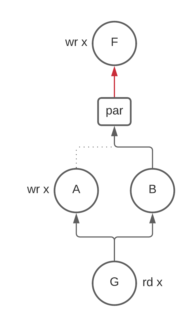
Par is the only statement that differs substantially from traditional dataflow because control flow graphs don't support nodes running in parallel. In other words, there is only ever one thing executing. However, par changes this and allows multiple things to execute at the same time. Consider the following example where we are computing the liveness of x to see why this is weird:

F; // wr x
...
par {
  A; // wr x
  B;
}
G; // rd x

Is x alive between X and the beginning of par? The answer is no because we know that both A and B will run. Therefore the write to x in F can not be seen by any group.

At first glance this doesn't seem like a problem. Great, we say, we can just take the union of the outputs of the children of par and call it a day.

This is wrong because B doesn't kill x and so x is alive coming into B. The union preserves this information and results in x being alive above par.

Taking the set intersection is not quite right here either. Consider adding another group C that reads from x.

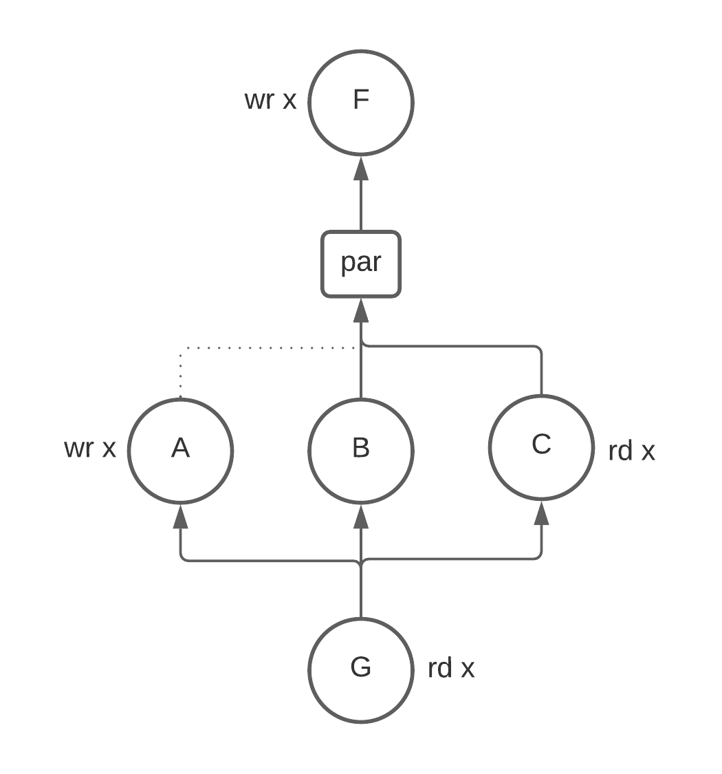
We have no information about how this read is ordered with the write to x in A so we have to assume that x is alive above par. If we take the intersection here:

  live(A) & live(B) & live(C)
= {} & {x} & {x}
= {}

We get the wrong answer. More generally, we can see that union clobbers any writes and intersection clobbers any reads that happen in the par.

The solution to this problem is solved by passing the gen and kill sets along with the live sets. Then par can set its output to be

(union(live(children)) - union(kill(children))) | union(gen(children))

The final tricky bit is thinking about how information flows between siblings in a par statement. Consider again the picture above with three nodes: A, B, and C. Should x be live at B? For liveness it turns out to be yes, but bare with me for a second for a thought experiment and consider the case where we have the guarantee that statements running in parallel can not interact with each other. This lets us reorder statements in some cases. Then there seems to be an information trade-off for how to define the liveness of x at B:

You could say that x is dead at B because it doesn't see any previous writes to x and doesn't read from x. This implies that you could potentially replace writes to other registers with x. However, this by itself would cause x to be written to twice in parallel. You would have to reorder B to run before A. The takeaway here is that calling x dead at B gives the register reuse pass more information to work with. To compute this information B needs the gens and kills from all of its siblings (for the same reason that par) needed it. This is not particularly hard to implement, but it's worthy of noting.
If you say that x is live at B, then you can never rewrite B to use x instead of some other register, but you also don't have to worry about reordering statements in a par.

Leaving thought experiment land, in our case we can never reorder statements in a par because siblings may interact with each other in arbitrary ways. For this reason, we must say that x is live at B. However, it's not immediately clear to me that this will be true of all dataflow analyses. That's why I set this thought experiment down in writing.

Equivalence to worklist algorithm

In the normal worklist algorithm, we add a statement back to the worklist when its predecessor has changed.

The intuition for why this algorithm is equivalent to worklist algorithm is that because the only entry into the children for each parent control statement is the parent control statement itself. The only way that a child statement would need to be recomputed is if the inputs to the parent need to be recomputed. Anything above the parent in the tree will take care of this re-computation.

Calyx Documentation